Analysis
1 Libraries
To reproduce the examples of this material, the R packages the following packages are needed.
library(EnvRtype)
library(rio)
library(ggh4x)
library(ggridges)
library(tidyverse)
library(metan)
library(lmerTest)
library(lme4)
library(broom)
library(broom.mixed)

my_theme <-
  theme_bw() +
  theme(panel.spacing = unit(0, "cm"),
        panel.grid = element_blank(),
        legend.position = "bottom")
2 Datasets
2.1 Traits
df_traits <-
  import("https://bit.ly/df_barley") |>
  as_factor(1:6)
2.2 Climate variables
2.2.1 Scripts to gather data
df_env <- import("https://bit.ly/3RvXlgj")
ENV <- df_env$env |> as_character()
LAT <- df_env$Lat
LON <- df_env$Lon
ALT <- df_env$Alt
START <- df_env$Sowing
END <- df_env$Harvesting

# see more at https://github.com/allogamous/EnvRtype
df_climate <-
  get_weather(env.id = ENV,
              lat = LAT,
              lon = LON,
              start.day = START,
              end.day = END)
# GDD: Growing Degree Day (oC/day)
# FRUE: Effect of temperature on radiation use efficiency (from 0 to 1)
# T2M_RANGE: Daily Temperature Range (oC day)
# SPV: Slope of saturation vapour pressure curve (kPa.Celsius)
# VPD: Vapour pressure deficit (kPa)
# ETP: Potential Evapotranspiration (mm.day)
# PEPT: Deficit by Precipitation (mm.day)
# n: Actual duration of sunshine (hour)
# N: Daylight hours (hour)
# RTA: Extraterrestrial radiation (MJ/m^2/day)
# SRAD: Solar radiation (MJ/m^2/day)
# T2M: Temperature at 2 Meters
# T2M_MAX: Maximum Temperature at 2 Meters
# T2M_MIN: Minimum Temperature at 2 Meters
# PRECTOT: Precipitation
# WS2M: Wind Speed at 2 Meters
# RH2M: Relative Humidity at 2 Meters
# T2MDEW: Dew/Frost Point at 2 Meters
# ALLSKY_SFC_LW_DWN: Downward Thermal Infrared (Longwave) Radiative Flux
# ALLSKY_SFC_SW_DWN: All Sky Insolation Incident on a Horizontal Surface
# ALLSKY_TOA_SW_DWN: Top-of-atmosphere Insolation
# [1] "env"       "ETP"       "GDD"         "PETP"      "RH2M"      "SPV"
# [8] "T2M"       "T2M_MAX"   "T2M_MIN"   "T2M_RANGE" "T2MDEW"    "VPD"

# Compute other parameters
env_data <-
  df_climate %>%
  as.data.frame() %>%
  param_temperature(Tbase1 = 5, # choose the base temperature here
                    Tbase2 = 28, # choose the base temperature here
                    merge = TRUE) %>%
  param_atmospheric(merge = TRUE) %>%
  param_radiation(merge = TRUE)
2.2.2 Tidy climate data
env_data <- import("https://bit.ly/env_data_nasapower")
str(env_data)
## 'data.frame':    337 obs. of  19 variables:
##  $ env          : int  2019 2019 2019 2019 2019 2019 2019 2019 2019 2019 ...
##  $ LON          : num  30.5 30.5 30.5 30.5 30.5 ...
##  $ LAT          : num  31.1 31.1 31.1 31.1 31.1 ...
##  $ YEAR         : int  2019 2019 2019 2019 2019 2019 2019 2019 2019 2019 ...
##  $ MM           : int  11 11 11 11 11 11 11 11 11 11 ...
##  $ DD           : int  12 13 14 15 16 17 18 19 20 21 ...
##  $ DOY          : int  316 317 318 319 320 321 322 323 324 325 ...
##  $ YYYYMMDD     : chr  "12/11/2019" "13/11/2019" "14/11/2019" "15/11/2019" ...
##  $ daysFromStart: int  1 2 3 4 5 6 7 8 9 10 ...
##  $ tmean        : num  24.6 24.4 23.2 22.4 21.4 ...
##  $ tmax         : num  33.5 32.8 29.9 27.6 26.9 ...
##  $ tmin         : num  18 17.1 17.9 19.1 17.2 ...
##  $ prec         : num  0 0 0.05 0.06 0.06 0.01 0 0 0 0 ...
##  $ rh           : num  49.1 53.8 51.1 60.6 64.4 ...
##  $ trange       : num  15.52 15.68 11.97 8.45 9.77 ...
##  $ vpd          : num  2.42 2.11 1.79 1.38 1.17 ...
##  $ svpc         : num  0.196 0.188 0.178 0.173 0.162 ...
##  $ etp          : num  6.77 6.58 6.28 6.23 6.09 ...
##  $ dbp          : num  -6.77 -6.58 -6.23 -6.17 -6.03 ...
id_var <- names(env_data)[10:19]
3 Scripts
3.1 Correlation analysis of climate variables
env_data |>
  select_cols(all_of(id_var)) |>
  corr_coef() |>
  network_plot(min_cor = 0.3,
legend_position = "bottom") 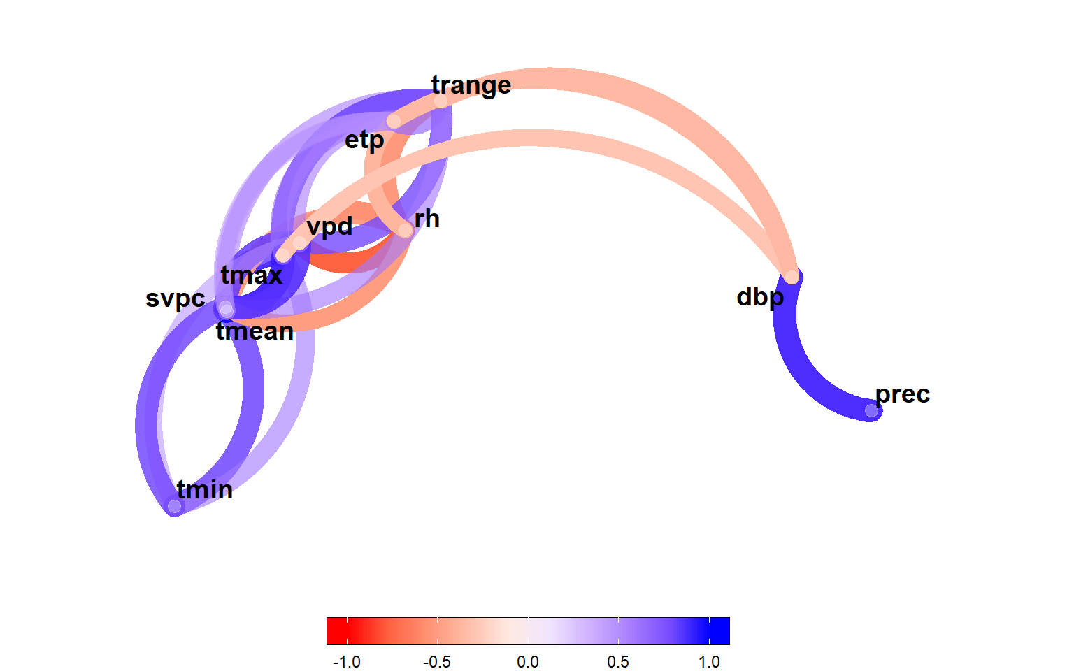
ggsave("figs/fig1_network.png", width = 5, height = 5)3.2 Distribution of climate variables
# long format for climate data
env_data_d <-
  env_data |>
  remove_cols(LON:YYYYMMDD, daysFromStart) |>
  pivot_longer(-env)

# long format for grain yield
df_gy_dist <-
  df_traits |>
  select(YEARS, GY) |>
  mutate(name = "GY", .after = YEARS) |>
  rename(value = GY,
         env = YEARS)
# bind climate and GY
env_data_d <- rbind(df_gy_dist, env_data_d)
# mean values for each trait
env_data_mean <- means_by(env_data_d, name)
ggplot(env_data_d, aes(x = value, y = env, fill = env)) +
geom_density_ridges(scale = 0.9) +
geom_vline(data = env_data_mean,
aes(xintercept = value),
linetype = 2) +
facet_grid(~name, scales = "free") +
theme(panel.grid.minor = element_blank(),
legend.position = "bottom",
legend.title = element_blank()) +
scale_y_discrete(expand = expansion(c(0, 0.05))) +
labs(x = "Observed value",
y = "Density",
fill = "") +
my_theme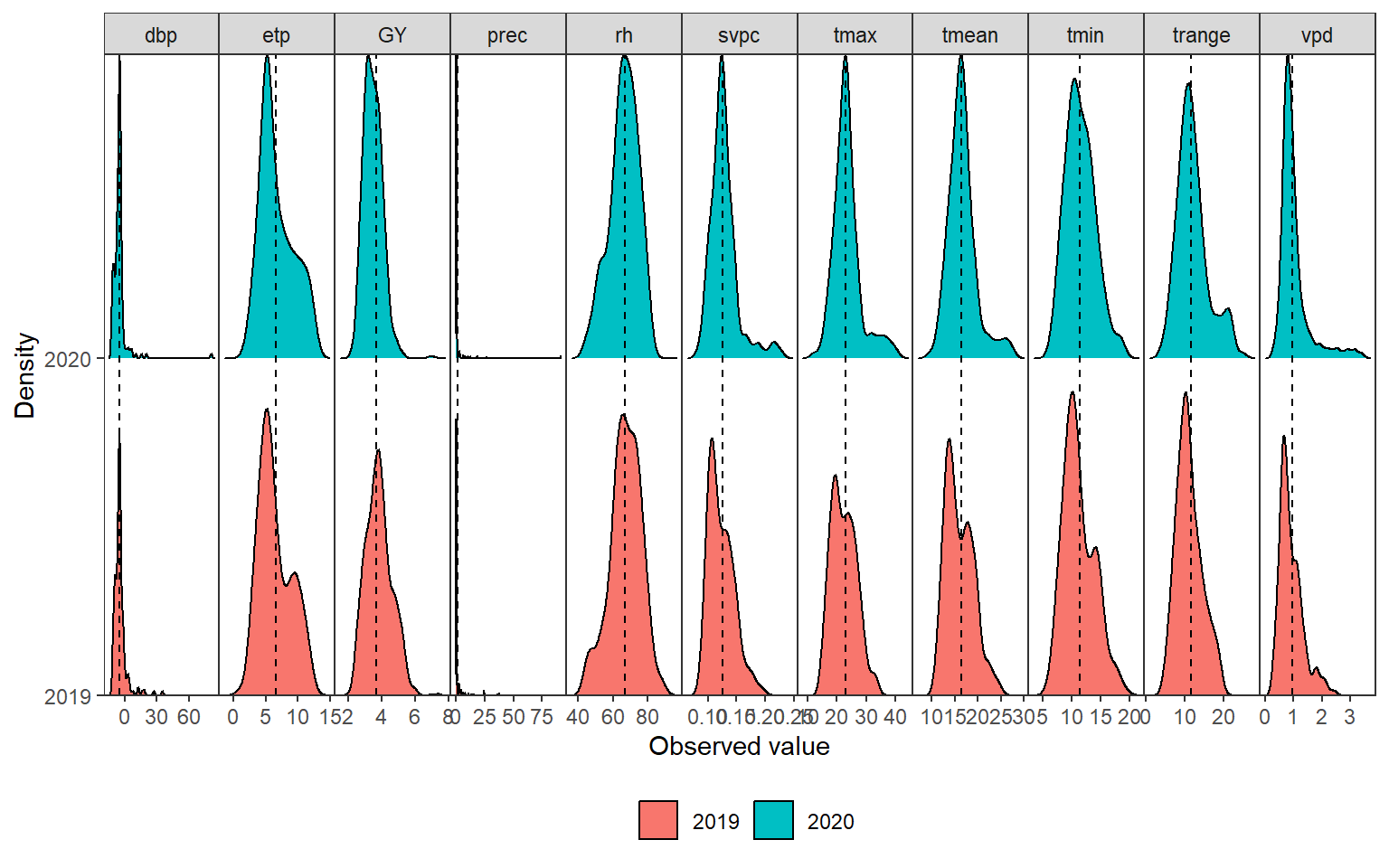
ggsave("figs/fig2_density_climate.png", width = 12, height = 5)3.3 Environmental tipology
names.window <- c('1-initial growing',
                  '2-Tillering',
                  '3-Booting',
                  '4-Heading/Flowering',
                  "5-Grain filling",
                  "6-Physiological maturity")

out <-
  env_typing(env.data = env_data,
             env.id = "env",
             var.id = c("trange", "tmax", "tmin", "dbp", "etp", "vpd"),
             by.interval = TRUE,
             time.window = c(0, 15, 35, 65, 90, 140),
             names.window = names.window)

out2 <-
  separate(out,
           env.variable,
           into = c("var", "freq"),
           sep = "_",
           extra = "drop")
3.3.1 tmax
# plot the distribution of envirotypes for dbp
p1 <-
  out2 |>
  subset(var == "tmax") |> # change the variable here
  ggplot() +
  geom_bar(aes(x=Freq, y=interval,fill=freq),
           position = "fill",
           stat = "identity",
           width = 1,
           color = "white",
           size=.2)+
  facet_grid(~env, scales = "free", space = "free")+
  scale_y_discrete(expand = c(0,0))+
  scale_x_continuous(expand = c(0,0))+
  xlab('Relative frequency of the maximum temperature (ºC)')+
  ylab("Crop stage")+
  labs(fill='Envirotype')+
  theme(axis.title = element_text(size=12),
        legend.text = element_text(size=9),
        strip.text = element_text(size=12),
        legend.title = element_text(size=12),
        strip.background = element_rect(fill="gray95",size=1),
        legend.position = 'bottom')
3.3.2 vpd
# plot the distribution of envirotypes for dbp

p2 <-
  out2 |>
  subset(var == "vpd") |> # change the variable here
  ggplot() +
  geom_bar(aes(x=Freq, y=interval,fill=freq),
           position = "fill",
           stat = "identity",
           width = 1,
           color = "white",
           size=.2)+
  facet_grid(~env, scales = "free", space = "free")+
  scale_y_discrete(expand = c(0,0))+
  scale_x_continuous(expand = c(0,0))+
  xlab(expression(Relative~frequency~of~the~vapor~pressure~deficit~~(KPa~day^{-1})))+
  ylab("Crop stage")+
  labs(fill='Envirotype')+
  theme(axis.title = element_text(size=12),
        legend.text = element_text(size=9),
        strip.text = element_text(size=12),
        legend.title = element_text(size=12),
        strip.background = element_rect(fill="gray95",size=1),
        legend.position = 'bottom')
3.3.3 dbp
# plot the distribution of envirotypes for dbp

p3 <-
  out2 |>
  subset(var == "dbp") |> # change the variable here
  ggplot() +
  geom_bar(aes(x=Freq, y=interval,fill=freq),
           position = "fill",
           stat = "identity",
           width = 1,
           color = "white",
           size=.2)+
  facet_grid(~env, scales = "free", space = "free")+
  scale_y_discrete(expand = c(0,0))+
  scale_x_continuous(expand = c(0,0))+
  xlab(expression(Relative~frequency~of~the~rainfall~deficit~~(mm~day^{-1})))+
  ylab("Crop stage")+
  labs(fill='Envirotype')+
  theme(axis.title = element_text(size=12),
        legend.text = element_text(size=9),
        strip.text = element_text(size=12),
        legend.title = element_text(size=12),
        strip.background = element_rect(fill="gray95",size=1),
        legend.position = 'bottom')


arrange_ggplot(p1, p2, p3,
               ncol = 1,
               tag_levels = "a")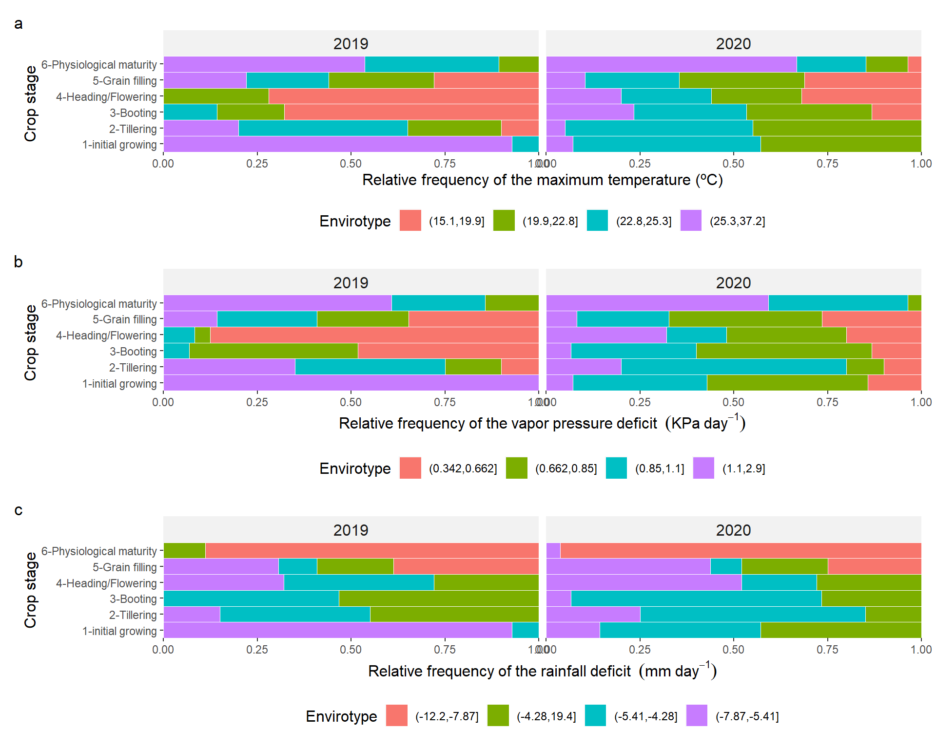
Figure 3.1: Quantiles for maximum temperature (a), vapor pressure deficit (b), and deficit by precipitation (c) across distinct crop stages of barley growing in two crop seasons.
ggsave("figs/fig3_typology.png", width = 10, height = 9)4 Analysis
4.1 Model
# Pivot longer to analyze each variable with group_by()
df_long <-
  df_traits |>
  pivot_longer(CAN:GY)

models <-
  df_long %>%
  group_by(YEARS, name) %>%
  doo(~lmer(value ~ STRESS + REP + (1|GENOTYPES) + (1|GENOTYPES:STRESS) + (1|REP:IBLOCK), data = .))
4.2 LRT
LRT <-
  models |>
  mutate(data = map(data,
                    ~.x %>%
                      lmerTest::ranova(., reduce.terms = TRUE) |>
                      rownames_to_column("term"))) |>
  unnest(data)
4.3 Variance components
vcomp <-
  models |>
  mutate(data = map(data,
                    ~.x %>%
                      lme4::VarCorr() |>
                      as.data.frame() |>
                      add_cols(Percent = (vcov / sum(vcov)) * 100))) |>
  unnest(data)


ggplot(vcomp, aes(name, vcov, fill = grp)) +
  geom_bar(stat = "identity",
           position = "fill",
           color = "black",
           width = 1) +
  facet_wrap(~YEARS) +
  geom_text(aes(label = paste0(round(Percent, 2), "%")),
            position = position_fill(vjust = .5),
            size = 3) +
  scale_y_continuous(expand = expansion(c(0, 0)),
                     labels = function(x) paste0(x*100, "%")) +
  scale_x_discrete(expand = expansion(0)) +
  theme_bw()+
  theme(legend.position = "bottom",
        axis.ticks.length = unit(0.2, "cm"),
        panel.grid = element_blank(),
        legend.title = element_blank(),
        strip.background = element_rect(fill = NA),
        text = element_text(colour = "black"),
        axis.text = element_text(colour = "black")) +
  labs(x = "Assessed traits",
       y = "Proportion of phenotypic variance")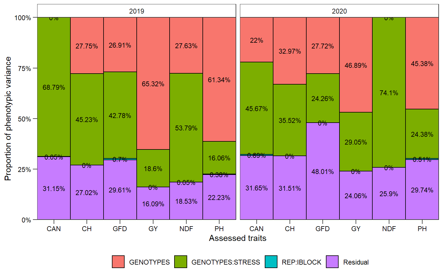
ggsave("figs/fig4_vcomp.png", width = 8, height = 6)5 BLUPs for Genotype x Stress by Year
blups <-
  models |>
  mutate(data = map(data,
                    ~.x %>%
                      augment())) |>
  unnest(data) |>
  group_by(YEARS, name, STRESS, GENOTYPES) |>
  summarise(blup = mean(.fitted)) |>
  ungroup() |>
  pivot_wider(names_from = name, values_from = blup)

blups
5.1 correlation between traits
cor_di <-
  blups |>
  filter(STRESS == "DI") |>
  corr_coef(CAN:PH) |>
  network_plot(legend_position = "bottom", show = "all")

cor_fi <-
  blups |>
  filter(STRESS == "FI") |>
  corr_coef(CAN:PH) |>
  network_plot(legend_position = "bottom", show = "all")

arrange_ggplot(cor_di, cor_fi,
               guides = "collect",
               tag_levels = "a")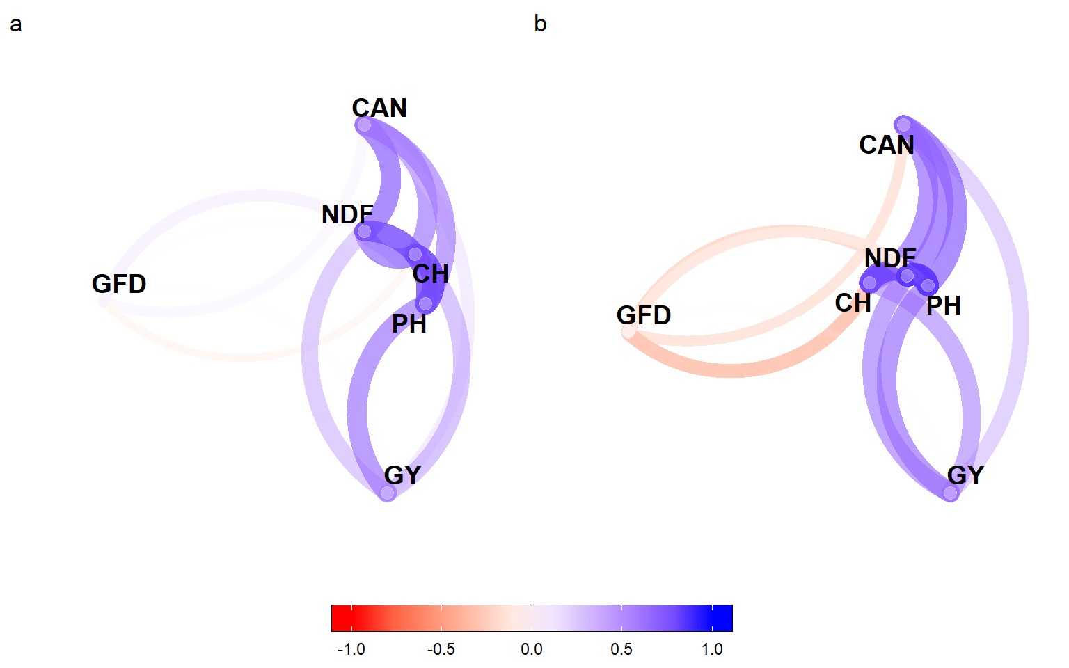
Figure 5.1: Correlation between traits under deficit irrigation (a) and full irrigation (b)
ggsave("figs/fig5_network_traits.png", width = 8, height = 5)6 MGIDI appied to each environment
blups_ys <- split_factors(blups, YEARS, STRESS)6.1 2019 DI
mgidi_2019_di <-
  blups_ys$`2019 | DI` |>
  column_to_rownames("GENOTYPES") |>
  mgidi(ideotype = c("l, h, h, h, l, h"),
        weights = c(1,1,1,5,1,2), # remove to consider equal heigths
        SI = 5,
        verbose = FALSE)
6.2 2019 FU
mgidi_2019_fi <-
  blups_ys$`2019 | FI` |>
  column_to_rownames("GENOTYPES") |>
  mgidi(ideotype = c("l, h, h, h, l, h"),
        weights = c(1,1,1,5,1,2), # remove to consider equal heigths
        SI = 5,
        verbose = FALSE)
6.3 2020 DI
mgidi_2020_di <-
  blups_ys$`2020 | DI` |>
  column_to_rownames("GENOTYPES") |>
  mgidi(ideotype = c("l, h, h, h, l, h"),
        weights = c(1,1,1,5,1,2), # remove to consider equal heigths
        SI = 5,
        verbose = FALSE)
6.4 2020 FU
mgidi_2020_fi <-
  blups_ys$`2020 | FI` |>
  column_to_rownames("GENOTYPES") |>
  mgidi(ideotype = c("l, h, h, h, l, h"),
        weights = c(1,1,1,5,1,2), # remove to consider equal heigths
        SI = 5,
        verbose = FALSE)
6.5 Selected genotypes
sel_2019DI <- mgidi_2019_di |> sel_gen()
sel_2019FI <- mgidi_2019_fi |> sel_gen()
sel_2020DI <- mgidi_2020_di |> sel_gen()
sel_2020FI <- mgidi_2020_fi |> sel_gen()

v1 <-
  venn_plot(sel_2019DI, sel_2020DI,
            sel_2019FI, sel_2020FI,
            names = c("2019DI", "2020DI", "2019FI", "2020FI"))


# Selected in DI
DI <- set_union(sel_2019DI, sel_2020DI)
# Selected in FI
FI <- set_union(sel_2019FI, sel_2020FI)


v2 <- venn_plot(DI, FI)
arrange_ggplot(v1, v2,
               tag_levels = "a")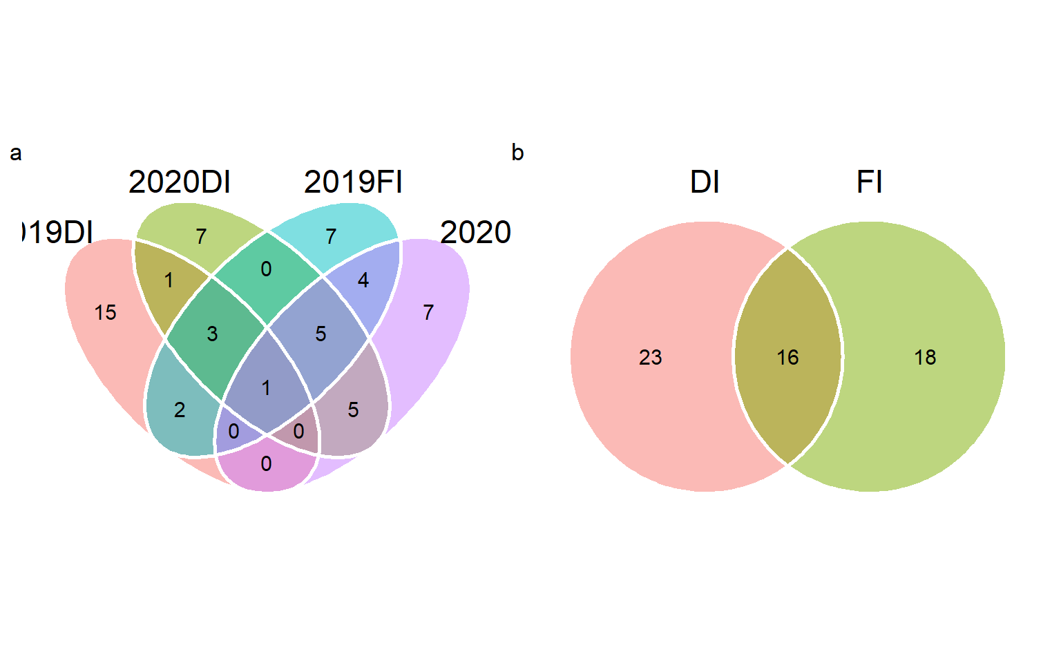
ggsave("figs/fig6_venn.png", width = 12, height = 5)

# only in DI (23)
set_difference(DI, FI)
##  [1] "08BA_82" "08AB_09" "06MT_91" "09BA_21" "08MT_63" "09AB_10" "07UT_46"
##  [8] "06WA_38" "08BA_95" "08MT_15" "07WA_03" "08MT_77" "08AB_46" "08AB_06"
## [15] "06MT_78" "06WA_53" "08WA_28" "08N2_66" "07UT_55" "09N2_74" "06WA_63"
## [22] "08WA_86" "07UT_14"

# only in FI (18)
set_difference(FI, DI)
##  [1] "09AB_89" "07AB_66" "08MT_68" "07AB_77" "07UT_94" "06MT_46" "07MT_43"
##  [8] "09AB_25" "09WA_19" "07BA_89" "09MT_16" "07UT_48" "08N6_90" "09AB_94"
## [15] "09AB_78" "06N2_39" "07UT_93" "08MT_10"


# in all environments
set_intersect(sel_2019DI, sel_2020DI, sel_2019FI, sel_2020FI)
## [1] "09UT_24"
6.6 MGIDI index for the selected genotypes
m1 <-
  gmd(mgidi_2019_di, "MGIDI") |>
  mutate(selected = ifelse(Genotype %in% set_union(sel_2019DI, sel_2020DI,
                                                   sel_2019FI, sel_2020FI),
                           "Yes",
                           "No")) |>
  subset(selected == "Yes") |>
  ggplot(aes(x = MGIDI, y = reorder(Genotype, -MGIDI))) +
  geom_line(aes(group = 1)) +
  geom_point(size = 2.5) +
  labs(x = "Multi-trait Genotype-Ideotype Distance Index",
       y = "Genotypes") +
  my_theme


m2 <-
  gmd(mgidi_2019_fi, "MGIDI") |>
  mutate(selected = ifelse(Genotype %in% set_union(sel_2019DI, sel_2020DI,
                                                   sel_2019FI, sel_2020FI),
                           "Yes",
                           "No")) |>
  subset(selected == "Yes") |>
  ggplot(aes(x = MGIDI, y = reorder(Genotype, -MGIDI))) +
  geom_line(aes(group = 1)) +
  geom_point(size = 2.5) +
  labs(x = "Multi-trait Genotype-Ideotype Distance Index",
       y = "Genotypes") +
  my_theme

m3 <-
  gmd(mgidi_2020_di, "MGIDI") |>
  mutate(selected = ifelse(Genotype %in% set_union(sel_2019DI, sel_2020DI,
                                                   sel_2019FI, sel_2020FI),
                           "Yes",
                           "No")) |>
  subset(selected == "Yes") |>
  ggplot(aes(x = MGIDI, y = reorder(Genotype, -MGIDI))) +
  geom_line(aes(group = 1)) +
  geom_point(size = 2.5) +
  labs(x = "Multi-trait Genotype-Ideotype Distance Index",
       y = "Genotypes") +
  my_theme

m4 <-
  gmd(mgidi_2020_fi, "MGIDI") |>
  mutate(selected = ifelse(Genotype %in% set_union(sel_2019DI, sel_2020DI,
                                                   sel_2019FI, sel_2020FI),
                           "Yes",
                           "No")) |>
  subset(selected == "Yes") |>
  ggplot(aes(x = MGIDI, y = reorder(Genotype, -MGIDI))) +
  geom_line(aes(group = 1)) +
  geom_point(size = 2.5) +
  labs(x = "Multi-trait Genotype-Ideotype Distance Index",
       y = "Genotypes") +
  my_theme

arrange_ggplot(m1, m2, m3, m4,
               ncol = 4,
               tag_levels = "a")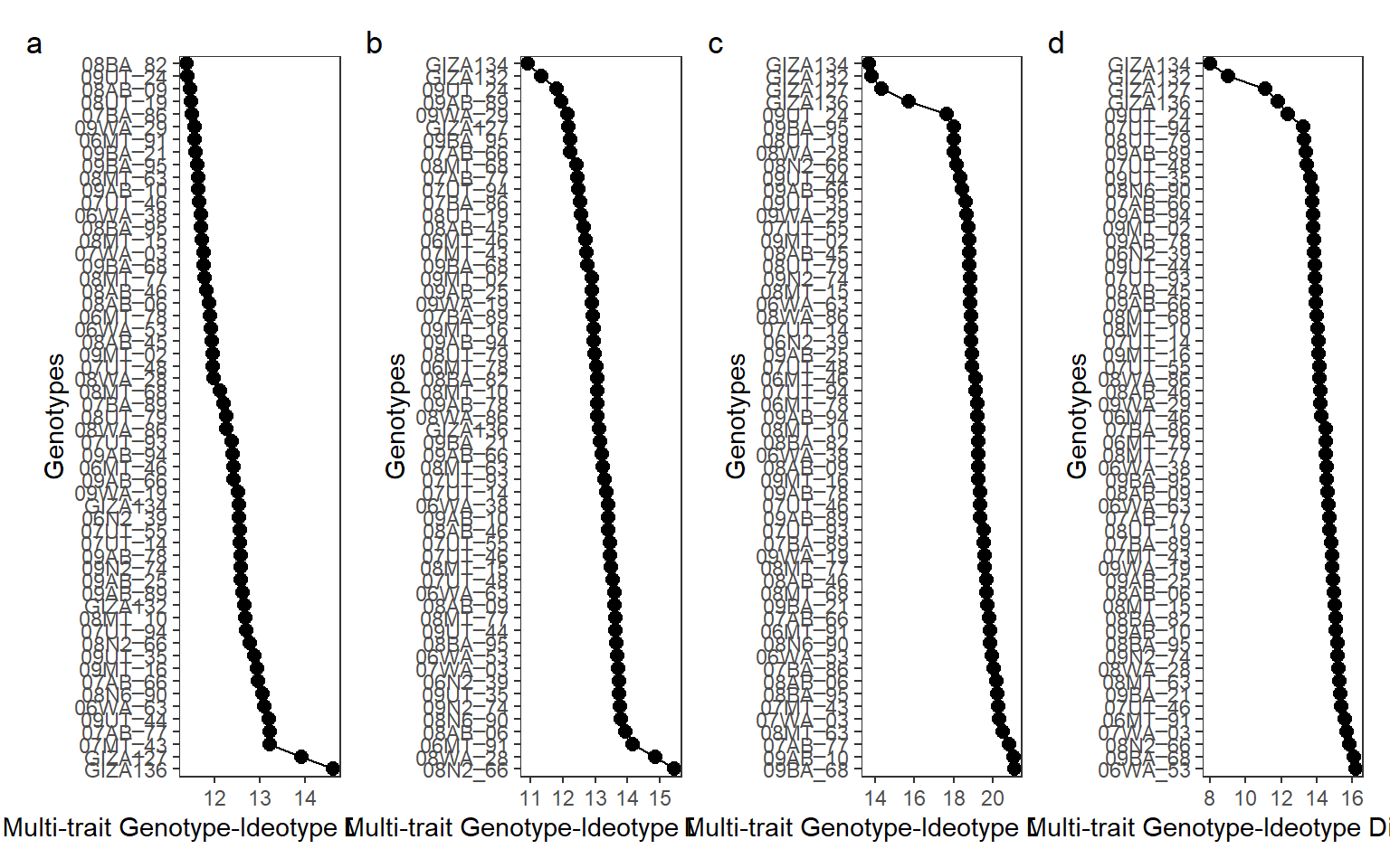
Figure 6.1: Selected genotypes ranked by the MGIDI in the environments 2019DI (a), 2020DI (b), 2019FI (c), and 2020FI (d)
ggsave("figs/fig7_selected.png", width = 17, height = 8)6.7 Selection gains
sel_gain <-
  list(
    a = gmd(mgidi_2019_di) |> mutate(YEAR = 2019, STRESS = "Deficit irrigation"),
    b = gmd(mgidi_2019_fi) |> mutate(YEAR = 2019, STRESS = "Full irrigation"),
    c = gmd(mgidi_2020_di) |> mutate(YEAR = 2020, STRESS = "Deficit irrigation"),
    d = gmd(mgidi_2020_fi) |> mutate(YEAR = 2020, STRESS = "Full irrigation")
  ) |>
  bind_rows() |>
  mutate(negative = ifelse(SDperc <= 0, "Negative", "Positive"))

library(ggh4x)

ggplot(sel_gain, aes(VAR, SDperc)) +
  geom_hline(yintercept = 0, size = 0.2) +
  geom_col(aes(fill = negative),
           col = "black",
           size = 0.2) +
  scale_y_continuous(expand = expansion(mult = 0.1)) +
  facet_nested(~YEAR + STRESS +sense, scales = "free", space = "free") +
  geom_text(aes(label = round(SDperc, 2),
                hjust = ifelse(SDperc > 0, -0.1, 1.1),
                angle = 90),
            size = 3) +
  labs(x = "Traits",
       y = "Selection gains (%)") +
  my_theme +
  theme(legend.position = "bottom",
        legend.title = element_blank(),
        panel.grid.minor = element_blank(),
        strip.background = element_rect(color = "black",
                                        fill = "white"))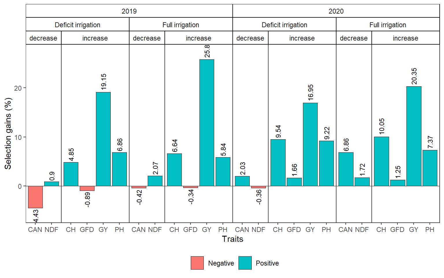
ggsave("figs/fig8_selection_gains.png", width = 12, height = 6)7 Section info
sessionInfo()
## R version 4.2.0 (2022-04-22 ucrt)
## Platform: x86_64-w64-mingw32/x64 (64-bit)
## Running under: Windows 10 x64 (build 22000)
##
## Matrix products: default
##
## locale:
## [1] LC_COLLATE=Portuguese_Brazil.utf8  LC_CTYPE=Portuguese_Brazil.utf8
## [3] LC_MONETARY=Portuguese_Brazil.utf8 LC_NUMERIC=C
## [5] LC_TIME=Portuguese_Brazil.utf8
##
## attached base packages:
## [1] stats     graphics  grDevices utils     datasets  methods   base
##
## other attached packages:
##  [1] broom.mixed_0.2.9.4 broom_1.0.0         lmerTest_3.1-3
##  [4] lme4_1.1-30         Matrix_1.4-1        metan_1.17.0.9000
##  [7] forcats_0.5.1       stringr_1.4.0       dplyr_1.0.9
## [10] purrr_0.3.4         readr_2.1.2         tidyr_1.2.0
## [13] tibble_3.1.7        tidyverse_1.3.1     ggridges_0.5.3
## [16] ggh4x_0.2.1         ggplot2_3.3.6       rio_0.5.29
## [19] EnvRtype_1.1.0
##
## loaded via a namespace (and not attached):
##  [1] nlme_3.1-157        fs_1.5.2            lubridate_1.8.0
##  [4] RColorBrewer_1.1-3  httr_1.4.3          numDeriv_2016.8-1.1
##  [7] tools_4.2.0         backports_1.4.1     bslib_0.3.1
## [10] utf8_1.2.2          R6_2.5.1            DBI_1.1.3
## [13] colorspace_2.0-3    withr_2.5.0         tidyselect_1.1.2
## [16] GGally_2.1.2        curl_4.3.2          compiler_4.2.0
## [19] textshaping_0.3.6   cli_3.3.0           rvest_1.0.2
## [22] xml2_1.3.3          labeling_0.4.2      bookdown_0.27
## [25] sass_0.4.1          scales_1.2.0        systemfonts_1.0.4
## [28] digest_0.6.29       minqa_1.2.4         foreign_0.8-82
## [31] rmarkdown_2.14      pkgconfig_2.0.3     htmltools_0.5.2
## [34] parallelly_1.32.0   highr_0.9           dbplyr_2.2.1
## [37] fastmap_1.1.0       rlang_1.0.3         readxl_1.4.0
## [40] rstudioapi_0.13     jquerylib_0.1.4     generics_0.1.3
## [43] farver_2.1.1        jsonlite_1.8.0      zip_2.2.0
## [46] magrittr_2.0.3      patchwork_1.1.1     Rcpp_1.0.8.3
## [49] munsell_0.5.0       fansi_1.0.3         furrr_0.3.1
## [52] lifecycle_1.0.1     stringi_1.7.6       yaml_2.3.5
## [55] mathjaxr_1.6-0      MASS_7.3-57         plyr_1.8.7
## [58] grid_4.2.0          parallel_4.2.0      listenv_0.8.0
## [61] ggrepel_0.9.1       crayon_1.5.1        lattice_0.20-45
## [64] haven_2.5.0         splines_4.2.0       hms_1.1.1
## [67] knitr_1.39          pillar_1.8.0        boot_1.3-28
## [70] reshape2_1.4.4      codetools_0.2-18    reprex_2.0.1
## [73] glue_1.6.2          evaluate_0.15       data.table_1.14.2
## [76] modelr_0.1.8        foreach_1.5.2       nloptr_2.0.3
## [79] vctrs_0.4.1         rmdformats_1.0.4    tzdb_0.3.0
## [82] tweenr_1.0.2        cellranger_1.1.0    gtable_0.3.0
## [85] polyclip_1.10-0     future_1.26.1       reshape_0.8.9
## [88] assertthat_0.2.1    xfun_0.31           ggforce_0.3.3
## [91] openxlsx_4.2.5      ragg_1.2.2          iterators_1.0.14
## [94] globals_0.15.1      ellipsis_0.3.2