Analysis
1 Installing pliman
To install the released version of pliman from CRAN type:
install.packages("pliman")The latest development version of pliman can be installed from the GitHub repository. The installation process requires the devtools package, which needs to be installed first. If you are a Windows user, you should also first download and install the latest version of Rtools.
if(!require(devtools)) install.packages("devtools")After devtools is properly installed, you can install pliman by running the following code. Please, note that the installation will also download the dependencies required to run the package.
devtools::install_github("TiagoOlivoto/pliman")Them, load pliman by running
library(pliman)2 Packages
library(pliman)     # plant image analysis
library(tidyverse)  # data manipulation and plots
# -- Attaching packages --------------------------------------- tidyverse 1.3.1 --
# v ggplot2 3.3.5     v purrr   0.3.4
# v tibble  3.1.4     v dplyr   1.0.7
# v tidyr   1.1.3     v stringr 1.4.0
# v readr   2.0.2     v forcats 0.5.1
# -- Conflicts ------------------------------------------ tidyverse_conflicts() --
# x dplyr::filter() masks stats::filter()
# x dplyr::lag()    masks stats::lag()
library(patchwork)  # plot arrangement
library(DescTools)  # concordance correlation coefficient
library(rio)        # import/export data
library(ggthemes)   # Themes for ggplot2
library(GGally)     # create pairwise ggplots
# Registered S3 method overwritten by 'GGally':
#   method from
#   +.gg   ggplot2
3 Helper functions
# concordance correlation coefficient
get_ccc <- function(df, predicted, real){
  if(is.grouped_df(df)){
    df %>%
      group_modify(~get_ccc(.x, {{predicted}}, {{real}})) %>%
      ungroup()
  } else{
    predicted <- pull(df, {{predicted}})
    real <- pull(df, {{real}})
    cor <- CCC(real, predicted, na.rm = TRUE)
    data.frame(r = cor(real, predicted),
               pc = cor$rho.c[[1]],
               lwr_ci = cor$rho.c[[2]],
               upr_ci = cor$rho.c[[3]],
               bc = cor$C.b)
  }
}


# helper function to plot the CCC in ggpairs()
custom_ccc <- function(data, mapping,...){
  data2 <- data
  data2$x <- as.numeric(data[,as_label(mapping$x)])
  data2$y <- as.numeric(data[,as_label(mapping$y)])
  data2$group <- data[,as_label(mapping$colour)]
  correlation_df <- data2 %>%
    group_by(group) %>%
    summarize(estimate = round(as.numeric(DescTools::CCC(x, y)$rho.c[1]),2))
  ggplot(data=correlation_df, aes(x=1,y=group, color = group))+
    geom_text(aes(label = paste0("rho[c]: ", estimate)),
              data = correlation_df,
              parse = TRUE,
              size = 4)
}
custom_smoth <- function(data, mapping, method="lm", ...){
  p <- ggplot(data = data, mapping = mapping) +
    geom_point(alpha = 0.7,
               shape = 21,
               size = 2.5,
               stroke = 0.01,
               color = "black") +
    geom_abline(color = "red",
                intercept = 0,
                size = 0.7,
                slope = 1,
                linetype = 2)
  p
}

# set the ggplot2 theme
theme_set(theme_bw())
4 User effect on palette selection
4.1 Disease
4.1.1 Bean angular spot
sev_bean_1 <-
  measure_disease(pattern = "F",
                  img_healthy = "h1",
                  img_symptoms = "s1",
                  img_background = "b1",
                  dir_original = "data/01-bean-angular-spot/originals",
                  parallel = TRUE)
sev_bean_2 <-
  measure_disease(pattern = "F",
                  img_healthy = "h2",
                  img_symptoms = "s2",
                  img_background = "b2",
                  dir_original = "data/01-bean-angular-spot/originals",
                  parallel = TRUE)
sev_bean_3 <-
  measure_disease(pattern = "F",
                  img_healthy = "h3",
                  img_symptoms = "s3",
                  img_background = "b3",
                  dir_original = "data/01-bean-angular-spot/originals",
                  parallel = TRUE)
sev_bean_4 <-
  measure_disease(pattern = "F",
                  img_healthy = "h4",
                  img_symptoms = "s4",
                  img_background = "b4",
                  dir_original = "data/01-bean-angular-spot/originals",
                  parallel = TRUE)

bind_bean <-
  bind_cols(sev_bean_1 %>% select(1,3) %>% rename(r1 = symptomatic),
            sev_bean_2 %>% select(3) %>% rename(r2 = symptomatic),
            sev_bean_3 %>% select(3) %>% rename(r3 = symptomatic),
            sev_bean_4 %>% select(3) %>% rename(r4 = symptomatic)) %>%
  mutate(disease = "Bean angular spot", .before = 1)
4.1.2 Rice brown spot
sev_rice_1 <-
  measure_disease(pattern = "F24",
                  img_healthy = "h1",
                  img_symptoms = "s1",
                  img_background = "b1",
                  dir_original = "data/02-rice-brownspot/originals",
                  dir_processed = "test",
                  save_image = TRUE,
                  parallel = TRUE)
sev_rice_2 <-
  measure_disease(pattern = "F",
                  img_healthy = "h2",
                  img_symptoms = "s2",
                  img_background = "b2",
                  dir_original = "data/02-rice-brownspot/originals",
                  parallel = TRUE)
sev_rice_3 <-
  measure_disease(pattern = "F",
                  img_healthy = "h3",
                  img_symptoms = "s3",
                  img_background = "b3",
                  dir_original = "data/02-rice-brownspot/originals",
                  parallel = TRUE)

sev_rice_4 <-
  measure_disease(pattern = "F",
                  img_healthy = "h4",
                  img_symptoms = "s4",
                  img_background = "b4",
                  dir_original = "data/02-rice-brownspot/originals",
                  parallel = TRUE)

bind_rice <-
  bind_cols(sev_rice_1 %>% select(1,3) %>% rename(r1 = symptomatic),
            sev_rice_2 %>% select(3) %>% rename(r2 = symptomatic),
            sev_rice_3 %>% select(3) %>% rename(r3 = symptomatic),
            sev_rice_4 %>% select(3) %>% rename(r4 = symptomatic)) %>%
  mutate(disease = "Rice brown spot", .before = 1)
4.1.3 Wheat tan spot
sev_wheat_1 <-
  measure_disease(pattern = "F",
                  img_healthy = "h1",
                  img_symptoms = "s1",
                  img_background = "b1",
                  dir_original = "data/03-wheat-tanspot/originals",
                  parallel = TRUE)
sev_wheat_2 <-
  measure_disease(pattern = "F",
                  img_healthy = "h2",
                  img_symptoms = "s2",
                  img_background = "b2",
                  dir_original = "data/03-wheat-tanspot/originals",
                  parallel = TRUE)
sev_wheat_3 <-
  measure_disease(pattern = "F",
                  img_healthy = "h3",
                  img_symptoms = "s3",
                  img_background = "b3",
                  dir_original = "data/03-wheat-tanspot/originals",
                  parallel = TRUE)

sev_wheat_4 <-
  measure_disease(pattern = "F",
                  img_healthy = "h4",
                  img_symptoms = "s4",
                  img_background = "b4",
                  dir_original = "data/03-wheat-tanspot/originals",
                  parallel = TRUE)

bind_wheat <-
  bind_cols(sev_wheat_1 %>% select(1,3) %>% rename(r1 = symptomatic),
            sev_wheat_2 %>% select(3) %>% rename(r2 = symptomatic),
            sev_wheat_3 %>% select(3) %>% rename(r3 = symptomatic),
            sev_wheat_4 %>% select(3) %>% rename(r4 = symptomatic)) %>%
  mutate(disease = "Wheat tan spot", .before = 1)
4.1.4 Tobacco xylella
sev_tobacco_1 <-
  measure_disease(pattern = "F",
                  img_healthy = "h1",
                  img_symptoms = "s1",
                  img_background = "b1",
                  dir_original = "data/04-tobacco-xylella/originals",
                  parallel = TRUE)
sev_tobacco_2 <-
  measure_disease(pattern = "F",
                  img_healthy = "h2",
                  img_symptoms = "s2",
                  img_background = "b2",
                  dir_original = "data/04-tobacco-xylella/originals",
                  parallel = TRUE)
sev_tobacco_3 <-
  measure_disease(pattern = "F",
                  img_healthy = "h3",
                  img_symptoms = "s3",
                  img_background = "b3",
                  dir_original = "data/04-tobacco-xylella/originals",
                  parallel = TRUE)

sev_tobacco_4 <-
  measure_disease(pattern = "F",
                  img_healthy = "h4",
                  img_symptoms = "s4",
                  img_background = "b4",
                  dir_original = "data/04-tobacco-xylella/originals",
                  parallel = TRUE)

bind_tobacco <-
  bind_cols(sev_tobacco_1 %>% select(1,3) %>% rename(r1 = symptomatic),
            sev_tobacco_2 %>% select(3) %>% rename(r2 = symptomatic),
            sev_tobacco_3 %>% select(3) %>% rename(r3 = symptomatic),
            sev_tobacco_4 %>% select(3) %>% rename(r = symptomatic)) %>%
  mutate(disease = "Tobacco xylella", .before = 1)
4.1.5 Olive peacock eye
sev_olive_1 <-
  measure_disease(pattern = "F216",
                  img_healthy = "h1",
                  img_symptoms = "s1",
                  img_background = "b1",
                  dir_original = "data/05-olive-peacock-eye/originals",
                  parallel = TRUE)
sev_olive_2 <-
  measure_disease(pattern = "F216",
                  img_healthy = "h2",
                  img_symptoms = "s2",
                  img_background = "b2",
                  dir_original = "data/05-olive-peacock-eye/originals",
                  parallel = TRUE)
sev_olive_3 <-
  measure_disease(pattern = "F216",
                  img_healthy = "h3",
                  img_symptoms = "s3",
                  img_background = "b3",
                  dir_original = "data/05-olive-peacock-eye/originals",
                  parallel = TRUE)

sev_olive_4 <-
  measure_disease(pattern = "F216",
                  img_healthy = "h4",
                  img_symptoms = "s4",
                  img_background = "b4",
                  dir_original = "data/05-olive-peacock-eye/originals",
                  parallel = TRUE)

bind_olive <-
  bind_cols(sev_olive_1 %>% select(1,3) %>% rename(r1 = symptomatic),
            sev_olive_2 %>% select(3) %>% rename(r2 = symptomatic),
            sev_olive_3 %>% select(3) %>% rename(r3 = symptomatic),
            sev_olive_4 %>% select(3) %>% rename(r4 = symptomatic)) %>%
  mutate(disease = "Olive peacock eye", .before = 1)
4.1.6 Soybean rust
sev_soybean_1 <-
  measure_disease(pattern = "F",
                  img_healthy = "h1",
                  img_symptoms = "s1",
                  img_background = "b1",
                  dir_original = "data/06-soybean_rust/originals",
                  parallel = TRUE)
sev_soybean_2 <-
  measure_disease(pattern = "F",
                  img_healthy = "h2",
                  img_symptoms = "s2",
                  img_background = "b2",
                  dir_original = "data/06-soybean_rust/originals",
                  parallel = TRUE)
sev_soybean_3 <-
  measure_disease(pattern = "F",
                  img_healthy = "h3",
                  img_symptoms = "s3",
                  img_background = "b3",
                  dir_original = "data/06-soybean_rust/originals",
                  parallel = TRUE)

sev_soybean_4 <-
  measure_disease(pattern = "F",
                  img_healthy = "h4",
                  img_symptoms = "s4",
                  img_background = "b4",
                  dir_original = "data/06-soybean_rust/originals",
                  parallel = TRUE)

bind_soybean <-
  bind_cols(sev_soybean_1 %>% select(1,3) %>% rename(r1 = symptomatic),
            sev_soybean_2 %>% select(3) %>% rename(r2 = symptomatic),
            sev_soybean_3 %>% select(3) %>% rename(r3 = symptomatic),
            sev_soybean_4 %>% select(3) %>% rename(r4 = symptomatic)) %>%
  mutate(disease = "Soybean rust", .before = 1)
5 Concordance correlation coefficient
5.1 Validation of the pliman for severity prediction
df_ccc <- import("data/bind_severity.xlsx")
df_long <-
  df_ccc %>%
  pivot_longer(`User 1`:`Joint`,
               names_to = "User",
               values_to = "pliman")

# Concordance correlation coefficient
ccc <-
  df_long %>%
  group_by(disease, User) %>%
  get_ccc(pliman, APSAssess) %>%
  mutate(rho = paste0("rho[c]:~", round(pc, 2),
                      "[(",round(lwr_ci,2), "-",
                      round(upr_ci,2), ")]" ),
         bc = paste0("C[b]:~", round(bc, 2)),
         r = paste0("r:~~~", round(r, 2))) %>%
  rename(name = User)

#  export(ccc, "data/ccc.xlsx")
df_11 <-
  df_ccc %>%
  select(disease, APSAssess:Joint) %>%
  pivot_longer(`User 1`:Joint)

ggplot(df_11, aes(APSAssess, value)) +
  geom_point(alpha = 0.7,
             aes(fill = name),
             color = "black",
             shape = 21,
             size = 2.5,
             stroke = 0.02) +
  geom_abline(intercept = 0,
              slope = 1,
              linetype = 2,
              color = "blue") +
  facet_grid(name~disease) +
  geom_text(aes(label=rho),
            x = 2,
            y = 93,
            hjust = 0,
            size = 3,
            data = ccc,
            parse = TRUE) +
  geom_text(aes(label=bc),
            x = 2,
            y = 80,
            size = 3,
            hjust = 0,
            data = ccc,
            parse = TRUE) +
  geom_text(aes(label=r),
            x = 2,
            y = 70,
            size = 3,
            hjust = 0,
            data = ccc,
            parse = TRUE) +
  theme_bw() +
  scale_x_continuous(limits = c(0, 100)) +
  scale_y_continuous(limits = c(0, 100)) +
  scale_color_colorblind() +
  theme_bw(base_size = 14) +
  theme(axis.title = element_text(color = "black"),
        axis.text = element_text(color = "black"),
        axis.ticks.length = unit(0.2, "cm"),
        panel.grid = element_blank(),
        legend.position = "bottom",
        strip.background = element_rect(fill = NA),
        panel.spacing = unit(0, "cm"),
        legend.title = element_blank()) +
  labs(x = "Actual severity (%)",
       y = "pliman severity (%)")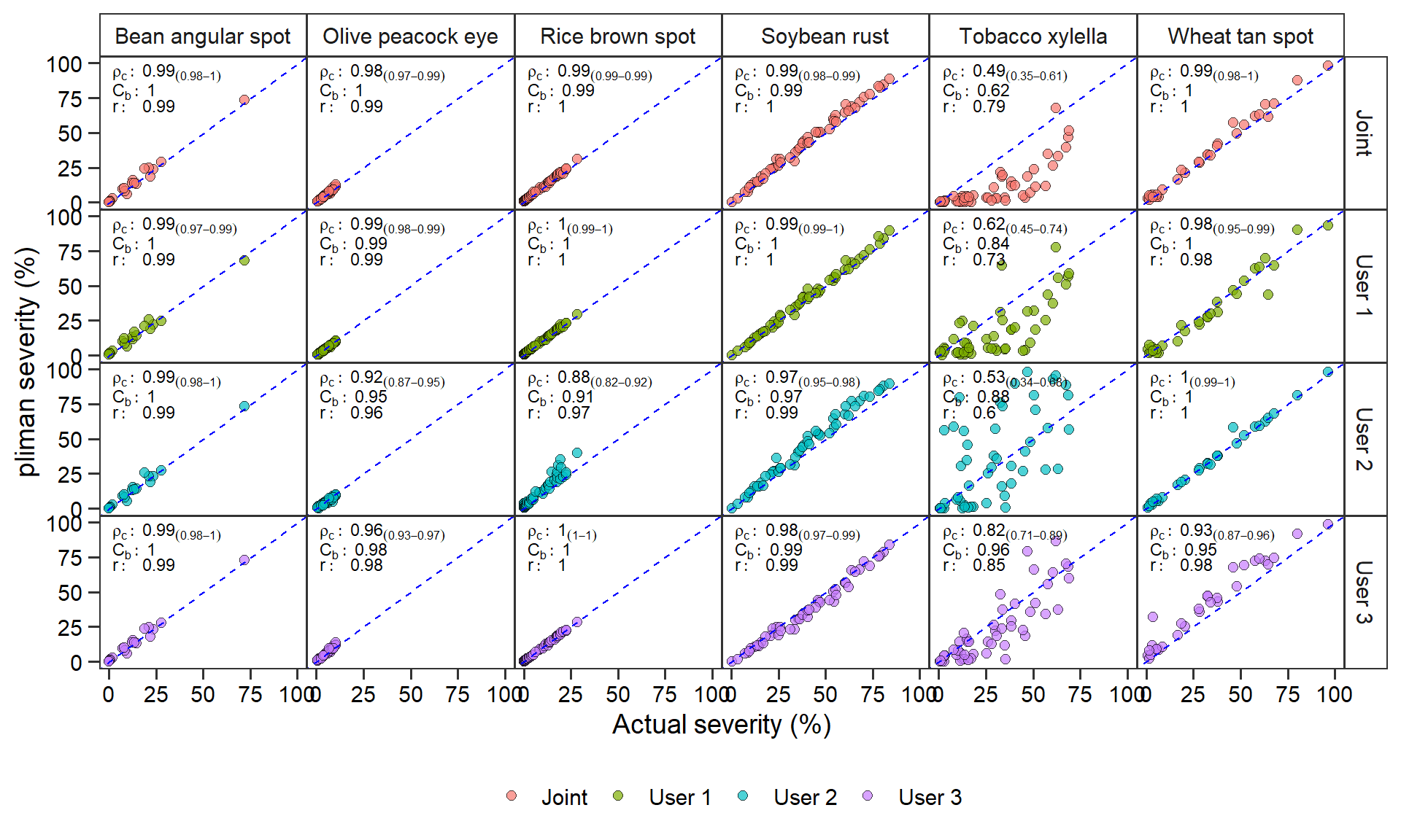
ggsave("figs/fig3_estimates.png", width = 10, height = 6, dpi = 600)5.2 Matrix of concordance correlation coefficients
df_ggpairs <-
  df_ccc %>%
  select(disease, ImageJ:APSAssess, Joint) %>%
  rename(pliman = Joint)
ggpairs(df_ggpairs,
        legend = 1,
        aes(color = disease, fill = disease),
        axisLabels = "none",
        columns = c("ImageJ", "LeafDoctor", "APSAssess", "pliman"),
        lower = list(continuous = custom_smoth),
        upper = list(continuous = custom_ccc),
        diag = list(continuous = wrap("densityDiag",
                                      alpha =  0.7,
                                      size = 0.2,
                                      color = "black"))) +
  scale_color_colorblind() +
  scale_fill_colorblind() +
  theme(panel.spacing = unit(0, "cm"),
        panel.grid = element_blank(),
        legend.position = "bottom",
        strip.background = element_rect(fill = NA),
        strip.text = element_text(size = 13),
        legend.title = element_blank())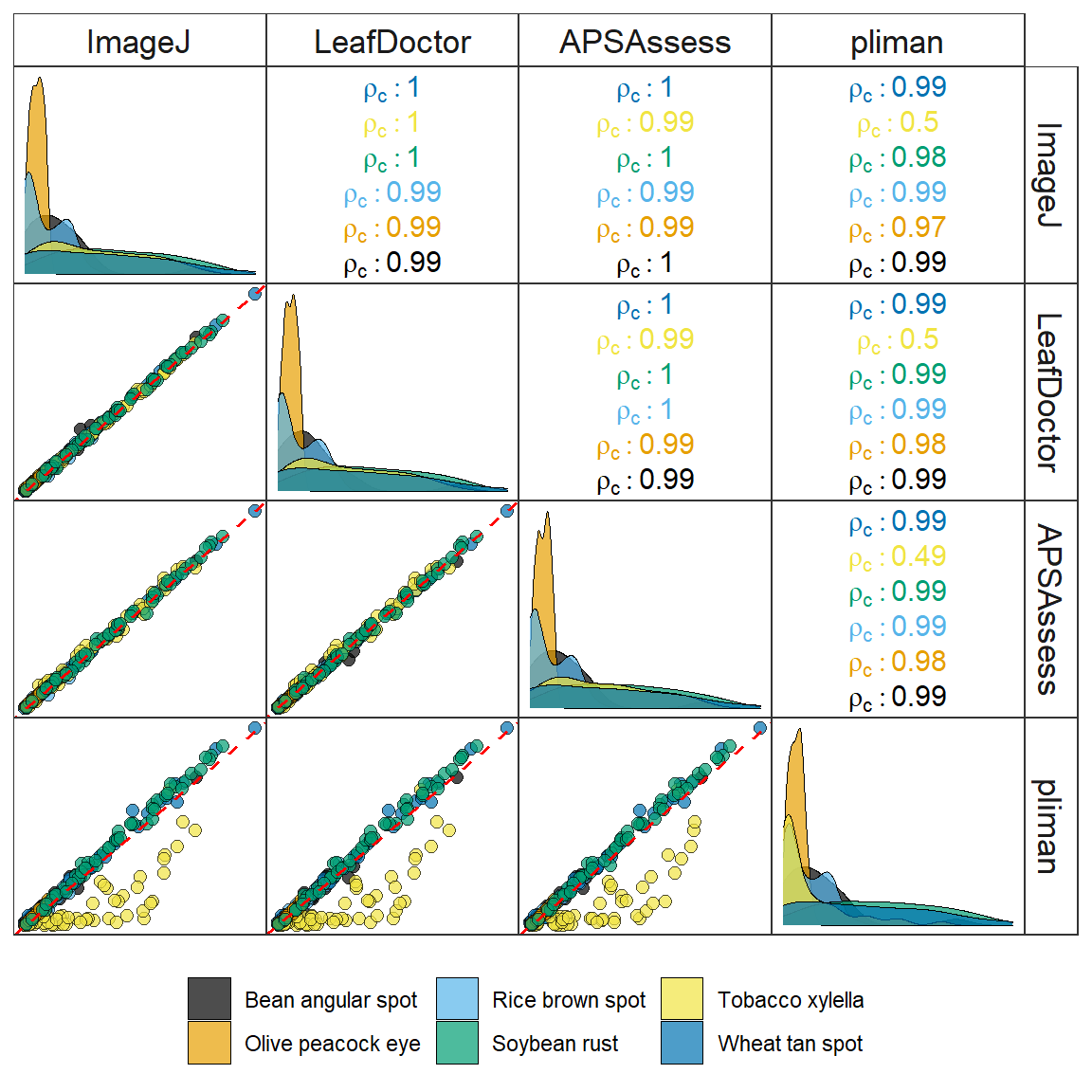
ggsave("figs/fig4_softwares.jpg", width = 6, height = 6, dpi = 600)6 Impact of image resolution on predicted severity
severity <- import("data/severity_scenario.xlsx")

# Concordance correlation coefficient by resolution
df_ccc_resolution <-
  severity %>%
  group_by(mp) %>%
  get_ccc(APSAssess, pliman) %>%
  mutate(rho = paste0("rho[c]:~", round(pc, 3),
                      "[(",round(lwr_ci,3), "-",
                      round(upr_ci,3), ")]" ),
         bco = paste0("C[b]:~", round(bc, 3)),
         rper = paste0("r:~~~", round(r, 3)))

p1 <-
  ggplot(severity, aes(APSAssess, pliman)) +
  geom_point(color = "black",
             size = 2,
             alpha = 0.25) +
  geom_abline(intercept = 0, slope = 1, linetype = 2, color = "red") +
  facet_wrap(~mp, ncol = 5) +
  geom_text(aes(label=rho),
            x = 2,
            y = 93,
            hjust = 0,
            size = 3,
            data = df_ccc_resolution,
            parse = TRUE) +
  geom_text(aes(label=bco),
            x = 2,
            y = 80,
            size = 3,
            hjust = 0,
            data = df_ccc_resolution,
            parse = TRUE) +
  geom_text(aes(label=rper),
            x = 2,
            y = 70,
            size = 3,
            hjust = 0,
            data = df_ccc_resolution,
            parse = TRUE) +
  scale_y_continuous(breaks = seq(0, 100, by = 25),
                     limits = c(0, 100)) +
  scale_x_continuous(breaks = seq(0, 100, by = 25),
                     limits = c(0, 100)) +
  coord_fixed() +
  theme(legend.background = element_blank(),
        panel.grid = element_blank(),
        panel.spacing = unit(0, "cm"),
        axis.title = element_text(color = "black"),
        axis.text = element_text(color = "black"),
        strip.background = element_rect(fill = NA),
        axis.ticks.length = unit(0.2, "cm")) +
  labs(x = "Actual severity (%)",
       y = "Predicted severity (%)")


p2 <-
  ggplot(severity, aes(residual)) +
  geom_density(aes(fill = factor(mp)), alpha = 0.3, size = 0.1) +
  geom_vline(xintercept = 0, linetype = 2) +
  geom_rug(length = unit(0.02, "npc"),
           size = 0.05,
           color = "gray") +
  theme(legend.position = "bottom",
        legend.title = element_blank(),
        panel.grid = element_blank(),
        panel.spacing = unit(0, "cm"),
        strip.background = element_rect(fill = NA),
        axis.title = element_text(color = "black"),
        axis.text = element_text(color = "black"),
        axis.ticks.length = unit(0.2, "cm")) +
  labs(x = "Prediction residual (%)") +
  scale_fill_colorblind()


df_ccc_resolution2 <-
  df_ccc_resolution %>%
  select(mp, r, pc, bc) %>%
  pivot_longer(-mp)

p3 <-
  ggplot(df_ccc_resolution2, aes(mp, value, fill = name, group = name)) +
  geom_line(aes(color = name)) +
  geom_point(shape = 21, size = 2) +
  theme(legend.position = "bottom",
        legend.title = element_blank(),
        panel.spacing = unit(0, "cm"),
        panel.grid = element_blank(),
        axis.title = element_text(color = "black"),
        axis.text = element_text(color = "black"),
        axis.ticks.length = unit(0.2, "cm")) +
  labs(x = "Image resolution (megapixel)",
       y = "Observed value") +
  scale_y_continuous(breaks = seq(0.9, 1, by = 0.002)) +
  scale_x_continuous(breaks = c(0.05, 0.4, 0.7, 1.7, 3)) +
  scale_fill_colorblind(labels = c(~C[b],~rho[c], ~r)) +
  scale_color_colorblind(labels = c(~C[b],~rho[c], ~r))

p1 / (p3 + p2 + plot_layout(widths = c(1, 1.1))) +
  plot_annotation(tag_levels = "a") +
  plot_layout(ncol = 1)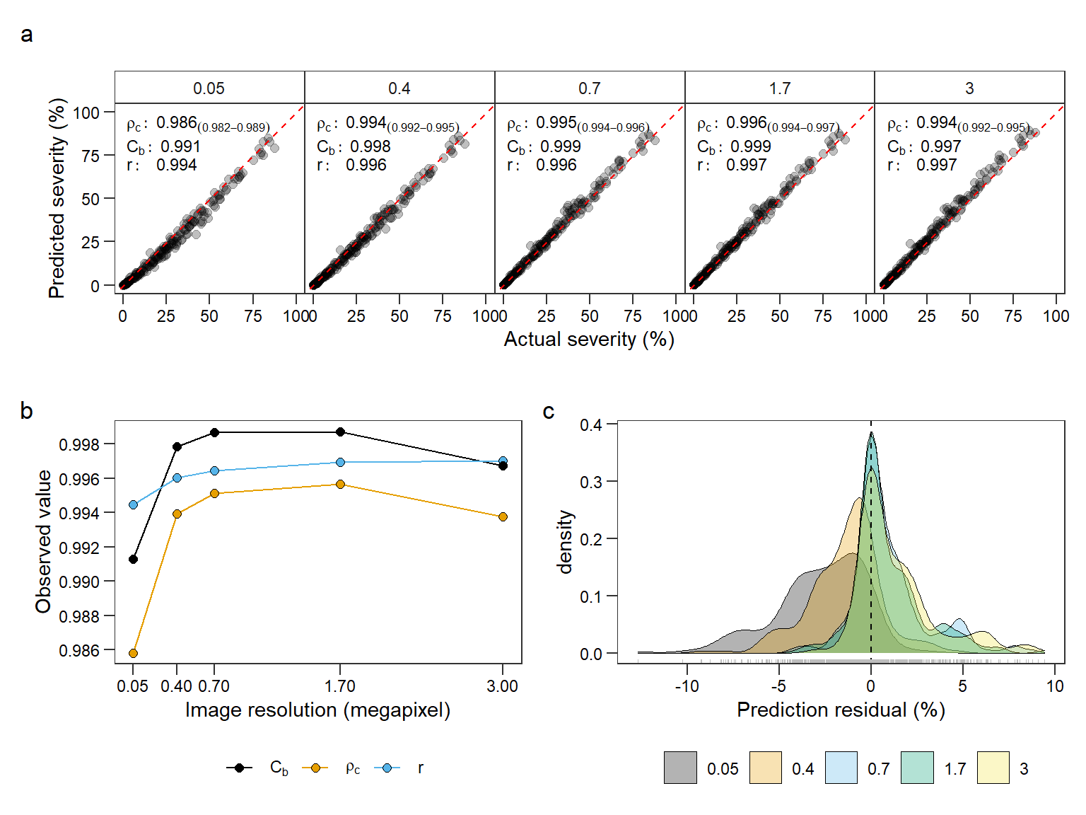
ggsave("figs/fig5_resolution.jpg", dpi = 600)
# Saving 8 x 6 in image
7 Computation time
scenario <- import("data/runtime_scenario.xlsx")
ggplot(scenario, aes(mp, elapsed_img, fill = strategy, group = strategy)) +
  geom_line(aes(color = strategy)) +
  geom_point(shape = 21, size = 2) +
  scale_y_continuous(breaks = seq(0, 3.5, by = 0.5),
                     limits = c(0, 3.5)) +
  scale_x_reverse(breaks = c(0.05, 0.4, 0.7, 1.7, 3)) +
  theme_bw(base_size = 14) +
  theme(legend.position = c(0.8, 0.8),
        legend.key=element_blank(),
        legend.box.background = element_blank(),
        legend.background = element_blank(),
        panel.grid = element_blank(),
        axis.title = element_text(color = "black"),
        axis.text = element_text(color = "black"),
        axis.ticks.length = unit(0.2, "cm")) +
  labs(x = "Image resolution",
       y = "Elapsed time (s)") +
  scale_fill_colorblind() +
  scale_color_colorblind()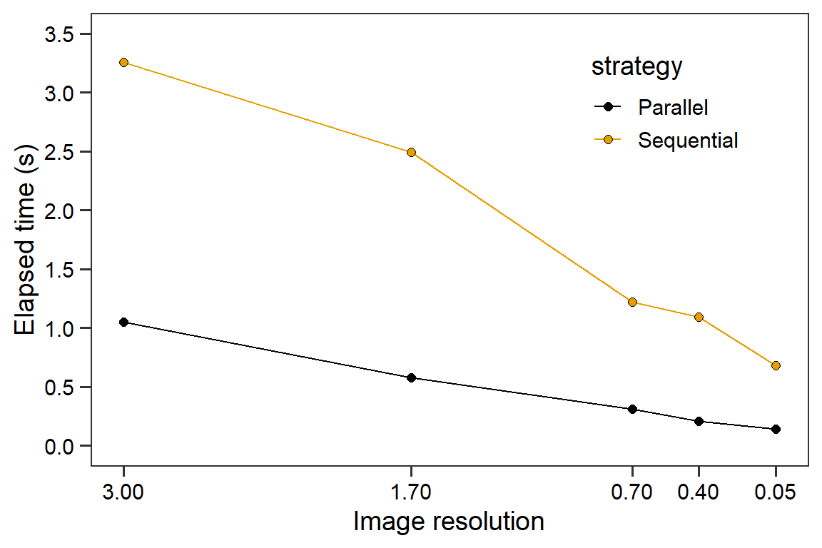
ggsave("figs/fig6_runningtime.png",
       width = 12,
       height = 9,
       units = "cm",
       dpi = 600)