Analysis
1 Libraries
To reproduce the examples of this material, the R packages the following packages are needed.
library(tidyverse)
library(EnvRtype)
library(metan)
library(rio)
library(factoextra)
library(FactoMineR)
library(ggrepel)
library(sp)
library(superheat)
library(corrr)

my_theme <-
  theme_bw() +
  theme(panel.spacing = unit(0, "cm"),
        panel.grid = element_blank(),
        legend.position = "bottom")
2 Datasets
2.1 Traits
me1 <- c("E3", "E4", "E5")
me2 <- c("E1", "E2", "E7")
me3 <- c("E6")
me4 <- c("E8")

df_traits <-
  import("https://bit.ly/df_traits_wheat") |>
  as_factor(1:6) |>
  mutate(me = case_when(ENV %in% me1 ~ "ME1",
                        ENV %in% me2 ~ "ME2",
                        ENV %in% me3 ~ "ME3",
                        ENV %in% me4 ~ "ME4"))
2.2 Climate variables
2.2.1 Scripts to gather data
df_env <- import("https://bit.ly/loc_info_wheat")
ENV <- df_env$ENV |> as_character()
LAT <- df_env$LAT
LON <- df_env$LON
ALT <- df_env$ALT
START <- df_env$START
END <- df_env$END

# see more at https://github.com/allogamous/EnvRtype
df_climate <-
  get_weather(env.id = ENV,
              lat = LAT,
              lon = LON,
              start.day = START,
              end.day = END)
# GDD: Growing Degree Day (oC/day)
# FRUE: Effect of temperature on radiation use efficiency (from 0 to 1)
# T2M_RANGE: Daily Temperature Range (oC day)
# SPV: Slope of saturation vapour pressure curve (kPa.Celsius)
# VPD: Vapour pressure deficit (kPa)
# ETP: Potential Evapotranspiration (mm.day)
# PEPT: Deficit by Precipitation (mm.day)
# n: Actual duration of sunshine (hour)
# N: Daylight hours (hour)
# RTA: Extraterrestrial radiation (MJ/m^2/day)
# SRAD: Solar radiation (MJ/m^2/day)
# T2M: Temperature at 2 Meters
# T2M_MAX: Maximum Temperature at 2 Meters
# T2M_MIN: Minimum Temperature at 2 Meters
# PRECTOT: Precipitation
# WS2M: Wind Speed at 2 Meters
# RH2M: Relative Humidity at 2 Meters
# T2MDEW: Dew/Frost Point at 2 Meters
# ALLSKY_SFC_LW_DWN: Downward Thermal Infrared (Longwave) Radiative Flux
# ALLSKY_SFC_SW_DWN: All Sky Insolation Incident on a Horizontal Surface
# ALLSKY_TOA_SW_DWN: Top-of-atmosphere Insolation
# [1] "env"       "ETP"       "GDD"         "PETP"      "RH2M"      "SPV"
# [8] "T2M"       "T2M_MAX"   "T2M_MIN"   "T2M_RANGE" "T2MDEW"    "VPD"

# Compute other parameters
env_data <-
  df_climate %>%
  as.data.frame() %>%
  param_temperature(Tbase1 = 5, # choose the base temperature here
                    Tbase2 = 28, # choose the base temperature here
                    merge = TRUE) %>%
  param_atmospheric(merge = TRUE) %>%
  param_radiation(merge = TRUE)
2.2.2 Tidy climate data
env_data <- import("https://bit.ly/df_climate_tidy")
str(env_data)
## 'data.frame':    991 obs. of  23 variables:
##  $ env          : chr  "E1" "E1" "E1" "E1" ...
##  $ LON          : num  -46.1 -46.1 -46.1 -46.1 -46.1 ...
##  $ LAT          : num  -19.4 -19.4 -19.4 -19.4 -19.4 ...
##  $ YEAR         : int  2018 2018 2018 2018 2018 2018 2018 2018 2018 2018 ...
##  $ MM           : int  5 5 5 5 5 5 5 5 5 5 ...
##  $ DD           : int  2 3 4 5 6 7 8 9 10 11 ...
##  $ DOY          : int  122 123 124 125 126 127 128 129 130 131 ...
##  $ YYYYMMDD     : chr  "05/02/2018" "05/03/2018" "05/04/2018" "05/05/2018" ...
##  $ daysFromStart: int  1 2 3 4 5 6 7 8 9 10 ...
##  $ tmean        : num  19.5 20 20.8 20.9 21.2 ...
##  $ tmax         : num  27.9 28.5 29.1 28.8 28.3 ...
##  $ tmin         : num  12.4 11.9 13.5 14.4 15 ...
##  $ prec         : num  0 0 0 0.03 0.15 0.09 0 0.02 0.02 0 ...
##  $ ws           : num  1.81 1.13 1.5 1.74 1.5 1.96 2.19 2.66 2.7 1.71 ...
##  $ rh           : num  64.3 67.7 65.8 71.6 70.3 ...
##  $ tdew         : num  11.5 12.9 13.2 14.8 14.9 ...
##  $ gdd          : num  15.1 14.9 15.8 16.2 16.5 ...
##  $ frue         : num  0.721 0.723 0.777 0.79 0.793 ...
##  $ trange       : num  15.5 16.6 15.6 14.5 13.3 ...
##  $ vpd          : num  1.24 1.15 1.27 1.11 1.08 ...
##  $ spv          : num  0.146 0.146 0.156 0.158 0.158 ...
##  $ etp          : num  9.34 8.71 9.12 9.09 8.05 ...
##  $ rta          : num  28.7 28.6 28.4 28.3 28.1 ...
id_var <- names(env_data)[10:23]
3 Scripts
3.1 Deviance analysis
3.1.1 Model
mod <-
  waasb(df_traits,
        env = ENV,
        gen = LINHAGEM,
        rep = BLOCO,
        resp = GY,
        wresp = 65) # maior peso para performance
## Evaluating trait GY |============================================| 100% 00:00:02
## ---------------------------------------------------------------------------
## P-values for Likelihood Ratio Test of the analyzed traits
## ---------------------------------------------------------------------------
##     model       GY
##  COMPLETE       NA
##       GEN 3.42e-03
##   GEN:ENV 1.60e-12
## ---------------------------------------------------------------------------
## All variables with significant (p < 0.05) genotype-vs-environment interaction

waasb_env <-
  mod$GY$model %>%
  select_cols(type, Code, Y, WAASB) %>%
  subset(type == "ENV") %>%
  remove_cols(type) %>%
  rename(env = Code)
3.1.2 BLUPs
blupge <- gmd(mod, "blupge")

blupge |>
  make_mat(GEN, ENV, GY) |>
kableExtra::kable()| E1 | E2 | E3 | E4 | E5 | E6 | E7 | E8 | |
|---|---|---|---|---|---|---|---|---|
| BRS264 | 5282.212 | 4375.401 | 4594.222 | 4309.549 | 4281.875 | 1388.500 | 4780.219 | 3097.102 |
| CD151 | 5133.199 | 3981.884 | 3926.679 | 3794.016 | 3484.885 | 1319.721 | 4620.826 | 2623.267 |
| ORS1403 | 4766.968 | 3736.375 | 4220.757 | 3889.708 | 3180.280 | 1257.991 | 4654.939 | 2338.469 |
| TBIOATON | 5245.098 | 4194.017 | 4931.574 | 4342.001 | 3907.777 | 1403.818 | 4381.267 | 3334.566 |
| TBIODUQUE | 4721.233 | 4002.825 | 4320.157 | 4029.873 | 3515.728 | 1194.683 | 4173.383 | 2472.263 |
| VI09004 | 5405.136 | 3823.713 | 4219.419 | 4673.127 | 3945.283 | 1567.313 | 4063.997 | 4068.188 |
| VI09007 | 5306.519 | 4077.755 | 4036.934 | 4251.391 | 3699.024 | 1348.749 | 3712.071 | 2862.309 |
| VI09031 | 5113.092 | 3957.394 | 4254.325 | 4028.081 | 3583.433 | 1515.600 | 3624.090 | 2929.144 |
| VI09037 | 5349.630 | 4144.215 | 3984.157 | 3818.913 | 3395.113 | 1322.178 | 4082.302 | 3068.612 |
| VI130679 | 4898.978 | 3482.268 | 4240.474 | 4341.289 | 3503.989 | 1290.447 | 4090.410 | 2681.753 |
| VI130755 | 4621.478 | 3607.496 | 4299.799 | 3979.093 | 3228.663 | 1536.910 | 4279.266 | 2956.022 |
| VI130758 | 4420.186 | 3883.127 | 4110.813 | 3996.567 | 3162.743 | 1465.386 | 4025.409 | 2915.004 |
| VI131313 | 4638.819 | 3365.552 | 4406.752 | 3928.296 | 3836.338 | 1027.820 | 4130.877 | 3607.132 |
| VI14001 | 4767.310 | 3882.658 | 4113.718 | 4005.160 | 3987.910 | 1274.379 | 4414.220 | 3260.650 |
| VI14022 | 5795.451 | 3893.188 | 3657.076 | 3906.779 | 3444.757 | 1409.069 | 4351.759 | 2821.162 |
| VI14026 | 5587.829 | 4356.687 | 4478.538 | 4073.389 | 3590.865 | 1644.671 | 4746.980 | 3500.302 |
| VI14050 | 5138.250 | 3740.847 | 4237.278 | 4146.238 | 3727.650 | 1120.703 | 3846.712 | 2737.465 |
| VI14055 | 5317.182 | 3807.208 | 4461.491 | 4550.300 | 3900.639 | 1305.823 | 4654.967 | 3782.046 |
| VI14088 | 4424.901 | 3853.661 | 4527.776 | 4318.089 | 3484.264 | 1447.740 | 4055.049 | 3289.226 |
| VI14118 | 5104.537 | 4268.634 | 4110.750 | 4387.661 | 3901.315 | 1460.524 | 4242.764 | 3212.279 |
| VI14127 | 5706.292 | 4364.241 | 4603.708 | 4747.488 | 3915.401 | 1740.892 | 4482.711 | 3393.733 |
| VI14194 | 5676.327 | 4162.057 | 4961.301 | 4398.171 | 3427.092 | 1629.539 | 4427.013 | 2851.565 |
| VI14197 | 5884.131 | 4282.643 | 4379.148 | 4424.835 | 3995.823 | 1551.573 | 4602.824 | 3402.922 |
| VI14204 | 5459.974 | 3703.244 | 4151.558 | 4351.972 | 3572.006 | 1646.681 | 4380.814 | 2555.760 |
| VI14208 | 5005.025 | 3947.994 | 4307.456 | 4315.366 | 3684.816 | 1439.680 | 4344.208 | 2242.330 |
| VI14214 | 5060.277 | 4182.438 | 4368.321 | 4813.690 | 3932.955 | 1467.075 | 4521.619 | 2750.499 |
| VI14239 | 4509.855 | 3706.111 | 3816.209 | 3738.575 | 3646.618 | 1090.055 | 3869.924 | 2648.904 |
| VI14327 | 5206.957 | 3838.772 | 4342.125 | 4467.298 | 3680.383 | 1304.019 | 4322.401 | 3075.899 |
| VI14426 | 4814.134 | 3970.362 | 3994.451 | 3881.549 | 3657.549 | 1469.320 | 4270.031 | 2844.000 |
| VI14668 | 5227.392 | 3898.227 | 4148.233 | 4154.099 | 3817.169 | 1671.475 | 4182.941 | 3525.416 |
| VI14708 | 4962.562 | 3870.104 | 4414.772 | 4199.288 | 3464.495 | 1191.188 | 4292.413 | 3077.765 |
| VI14774 | 4384.071 | 4211.409 | 4495.336 | 4339.294 | 3882.483 | 1745.971 | 4368.136 | 3800.955 |
| VI14867 | 4420.342 | 4165.921 | 4757.046 | 4198.044 | 3345.108 | 1515.569 | 4374.169 | 3551.408 |
| VI14881 | 4625.981 | 3964.294 | 4359.125 | 4332.484 | 3526.458 | 1232.242 | 3906.129 | 2712.908 |
| VI14950 | 4481.994 | 3748.665 | 3625.061 | 3651.642 | 3269.540 | 1178.599 | 3753.455 | 3360.014 |
| VI14980 | 4581.815 | 4252.448 | 4684.439 | 4616.686 | 3972.237 | 1448.636 | 4538.349 | 4093.405 |
3.1.3 BLUP-based stability
indexes <- blup_indexes(mod)
kableExtra::kable(indexes$GY)| GEN | Y | HMGV | HMGV_R | RPGV | RPGV_Y | RPGV_R | HMRPGV | HMRPGV_Y | HMRPGV_R | WAASB | WAASB_R |
|---|---|---|---|---|---|---|---|---|---|---|---|
| BRS264 | 4100.680 | 3399.344 | 9 | 1.0661581 | 3986.544 | 7 | 1.0629217 | 3974.442 | 6 | 4.411137 | 13 |
| CD151 | 3569.772 | 3069.257 | 27 | 0.9581046 | 3582.514 | 27 | 0.9530240 | 3563.516 | 27 | 6.472968 | 24 |
| ORS1403 | 3431.639 | 2937.676 | 32 | 0.9262602 | 3463.442 | 34 | 0.9172999 | 3429.938 | 34 | 8.474191 | 30 |
| TBIOATON | 4039.934 | 3391.916 | 10 | 1.0567667 | 3951.428 | 8 | 1.0551504 | 3945.384 | 8 | 3.645526 | 6 |
| TBIODUQUE | 3494.970 | 2955.484 | 31 | 0.9377248 | 3506.310 | 33 | 0.9320161 | 3484.964 | 33 | 4.967330 | 15 |
| VI09004 | 4044.224 | 3507.389 | 5 | 1.0743143 | 4017.041 | 5 | 1.0640415 | 3978.629 | 5 | 9.492961 | 33 |
| VI09007 | 3637.321 | 3140.779 | 23 | 0.9751691 | 3646.321 | 20 | 0.9716251 | 3633.069 | 20 | 6.223232 | 20 |
| VI09031 | 3589.642 | 3215.725 | 17 | 0.9772566 | 3654.126 | 19 | 0.9732532 | 3639.157 | 19 | 4.376393 | 11 |
| VI09037 | 3615.978 | 3121.602 | 25 | 0.9703666 | 3628.363 | 25 | 0.9674728 | 3617.543 | 23 | 5.990468 | 19 |
| VI130679 | 3511.346 | 3035.891 | 29 | 0.9468020 | 3540.251 | 30 | 0.9438644 | 3529.267 | 29 | 3.899486 | 7 |
| VI130755 | 3507.908 | 3187.475 | 20 | 0.9639141 | 3604.236 | 26 | 0.9600174 | 3589.666 | 26 | 4.604697 | 14 |
| VI130758 | 3420.731 | 3116.108 | 26 | 0.9449113 | 3533.182 | 31 | 0.9420777 | 3522.586 | 30 | 5.641056 | 18 |
| VI131313 | 3579.175 | 2912.168 | 34 | 0.9557968 | 3573.885 | 28 | 0.9391616 | 3511.683 | 31 | 8.741502 | 31 |
| VI14001 | 3705.031 | 3163.598 | 21 | 0.9904624 | 3703.505 | 18 | 0.9870455 | 3690.728 | 18 | 4.104274 | 9 |
| VI14022 | 3634.768 | 3145.821 | 22 | 0.9739454 | 3641.745 | 22 | 0.9670467 | 3615.950 | 24 | 10.242641 | 36 |
| VI14026 | 4079.307 | 3539.613 | 3 | 1.0772170 | 4027.895 | 4 | 1.0728824 | 4011.687 | 4 | 5.592509 | 17 |
| VI14050 | 3538.600 | 2935.837 | 33 | 0.9426835 | 3524.851 | 32 | 0.9366917 | 3502.447 | 32 | 4.384475 | 12 |
| VI14055 | 4046.443 | 3338.849 | 14 | 1.0559979 | 3948.553 | 9 | 1.0495848 | 3924.573 | 9 | 6.758444 | 25 |
| VI14088 | 3654.766 | 3243.731 | 16 | 0.9912060 | 3706.285 | 17 | 0.9875995 | 3692.800 | 17 | 7.181687 | 26 |
| VI14118 | 3866.786 | 3348.180 | 12 | 1.0289051 | 3847.249 | 13 | 1.0275836 | 3842.307 | 13 | 2.499678 | 2 |
| VI14127 | 4239.867 | 3670.072 | 1 | 1.1116878 | 4156.787 | 1 | 1.1091436 | 4147.274 | 1 | 5.031011 | 16 |
| VI14194 | 4005.844 | 3437.317 | 8 | 1.0544716 | 3942.846 | 10 | 1.0473564 | 3916.241 | 10 | 8.307873 | 29 |
| VI14197 | 4168.978 | 3534.048 | 4 | 1.0872193 | 4065.295 | 2 | 1.0857271 | 4059.715 | 2 | 6.309207 | 22 |
| VI14204 | 3724.131 | 3291.346 | 15 | 1.0028569 | 3749.850 | 15 | 0.9933115 | 3714.158 | 16 | 6.448952 | 23 |
| VI14208 | 3636.024 | 3126.078 | 24 | 0.9744482 | 3643.625 | 21 | 0.9625810 | 3599.252 | 25 | 8.188630 | 28 |
| VI14214 | 3934.028 | 3341.695 | 13 | 1.0364393 | 3875.420 | 12 | 1.0316511 | 3857.516 | 12 | 6.231577 | 21 |
| VI14239 | 3263.829 | 2808.385 | 36 | 0.8931993 | 3339.822 | 36 | 0.8891251 | 3324.588 | 36 | 3.265569 | 5 |
| VI14327 | 3792.597 | 3197.783 | 18 | 1.0023576 | 3747.983 | 16 | 1.0008608 | 3742.386 | 15 | 2.588900 | 3 |
| VI14426 | 3572.558 | 3190.599 | 19 | 0.9722236 | 3635.307 | 24 | 0.9703008 | 3628.117 | 21 | 3.081889 | 4 |
| VI14668 | 3856.329 | 3459.327 | 7 | 1.0411919 | 3893.191 | 11 | 1.0359063 | 3873.427 | 11 | 4.297511 | 10 |
| VI14708 | 3666.601 | 3064.466 | 28 | 0.9732026 | 3638.968 | 23 | 0.9701153 | 3627.424 | 22 | 1.819113 | 1 |
| VI14774 | 3955.560 | 3570.168 | 2 | 1.0711268 | 4005.122 | 6 | 1.0595827 | 3961.957 | 7 | 9.017335 | 32 |
| VI14867 | 3807.374 | 3356.203 | 11 | 1.0252543 | 3833.598 | 14 | 1.0177334 | 3805.476 | 14 | 9.578895 | 35 |
| VI14881 | 3532.752 | 3020.742 | 30 | 0.9498625 | 3551.695 | 29 | 0.9463929 | 3538.721 | 28 | 3.968622 | 8 |
| VI14950 | 3270.862 | 2900.714 | 35 | 0.9059717 | 3387.580 | 35 | 0.9004934 | 3367.096 | 35 | 8.053883 | 27 |
| VI14980 | 4113.677 | 3493.171 | 6 | 1.0845239 | 4055.216 | 3 | 1.0746910 | 4018.450 | 3 | 9.544612 | 34 |
3.1.4 GGE
mod_gge <- gge(blupge, ENV, GEN, GY, svp = 1)
p1 <-
  plot(mod_gge,
       size.text.gen = 2.5,
       size.text.env = 2.5) +
  my_theme

p2 <-
  plot(mod_gge,
       type = 2,
       size.text.gen = 2.5,
       size.text.env = 2.5) +
  my_theme

p3 <-
  plot(mod_gge,
       type = 3,
       size.text.gen = 2.5,
       size.text.env = 2.5,
       size.text.win = 3.5) +
  my_theme

p4 <-
  plot(mod_gge,
       type = 4,
       size.text.gen = 2.5,
       size.text.env = 2.5,
       size.text.win = 3.5) +
  my_theme

p5 <-
  plot(mod_gge,
       type = 6,
       size.text.gen = 2.5,
       size.text.env = 2.5,
       size.text.win = 3.5) +
  my_theme

p6 <-
  plot(mod_gge,
       type = 8,
       size.text.gen = 2.5,
       size.text.env = 2.5,
       size.text.win = 3.5) +
  my_theme

arrange_ggplot(p1, p2, p3, p4, p5, p6,
               ncol = 3,
               tag_levels = "a",
               guides = "collect")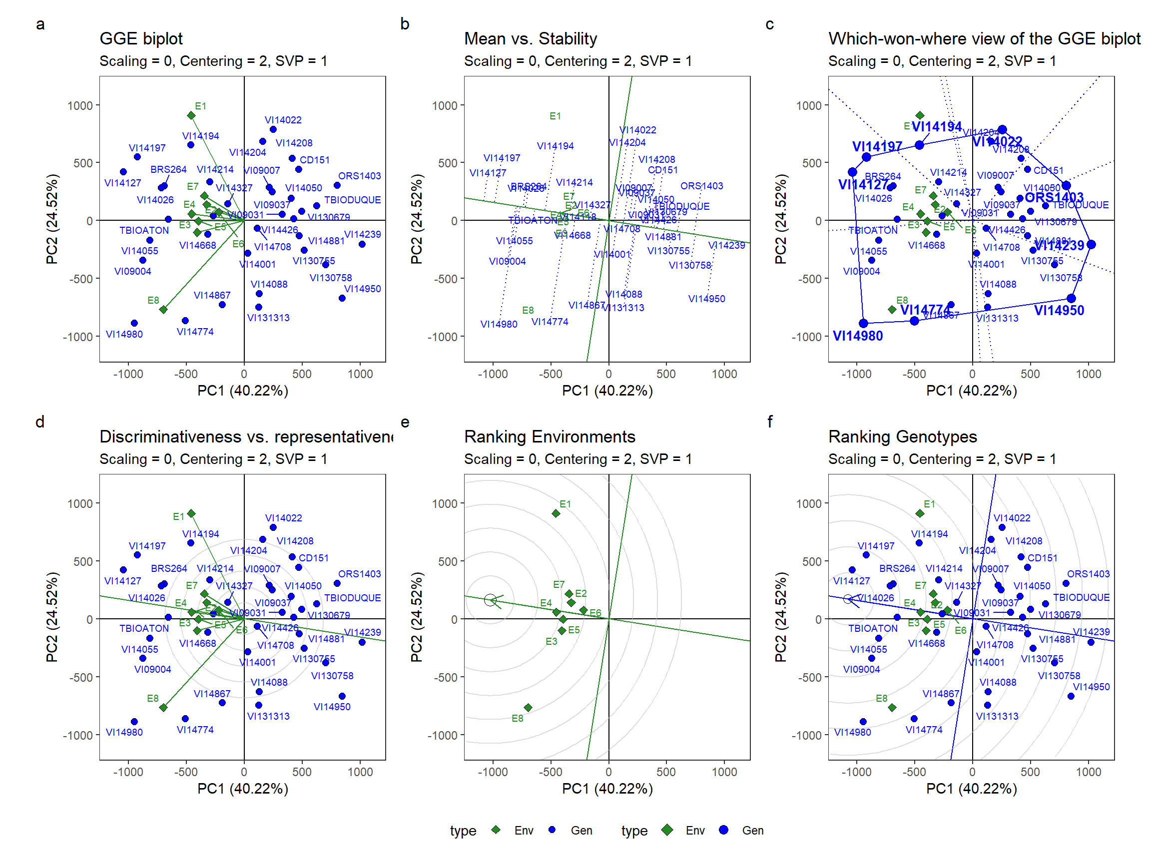
ggsave("figs/fig5_gge.png",
       width = 12,
       height = 9)
3.1.5 WAASBY
plot_waasby(mod, size.tex.lab = 6) +
  my_theme +
  theme(legend.position = c(0.8, 0.1))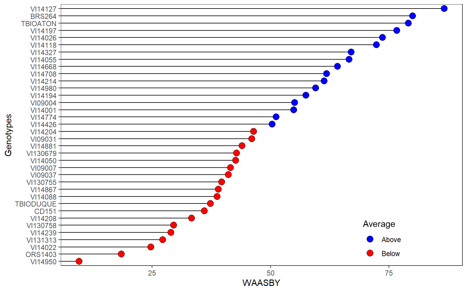
ggsave("figs/fig6_waasby.png",
       width = 5,
       height = 6)
3.2 Correlation between climate variables
env_data |>
  select_cols(tmean:rta) |>
  correlate() |>
  network_plot() +
  guides(color = guide_colorbar(barheight = 1,
                                barwidth = 20,
                                ticks.colour = "black")) +
  theme(legend.position = "bottom")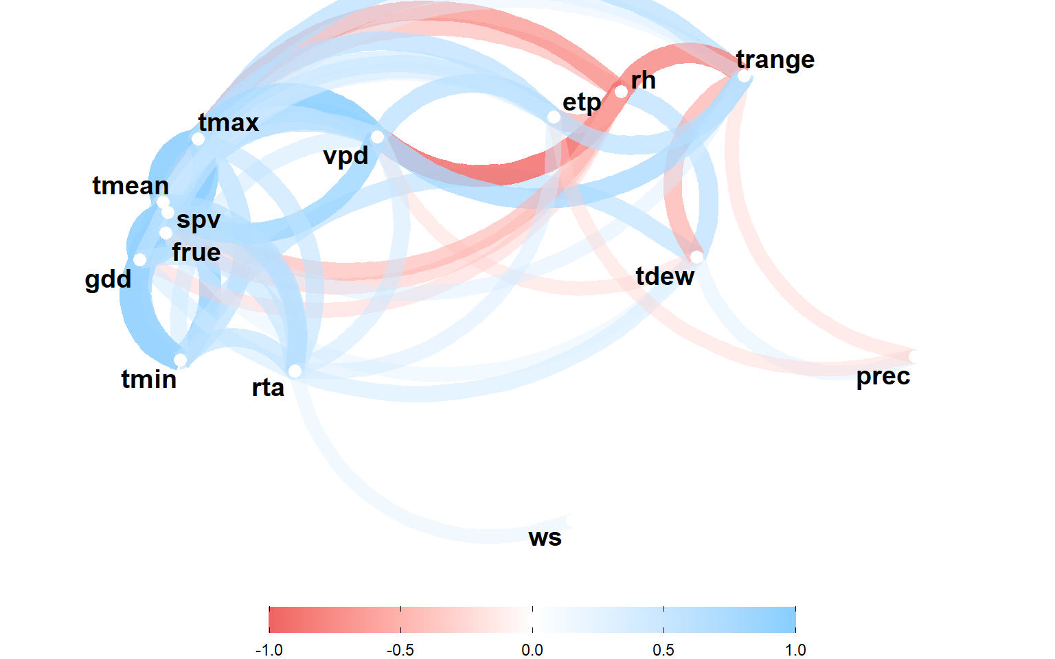
ggsave("figs/fig_network.png", width = 8, height = 8)3.3 Environmental kinships
EC <- W_matrix(env.data = env_data,
               by.interval = TRUE,
               statistic = 'quantile',
               time.window = c(0, 30, 55, 70, 95, 130))


distances <-
  env_kernel(env.data = EC,
             gaussian = TRUE)

d <-
  superheat(distances[[2]],
            heat.pal = c("#b35806", "white", "#542788"),
            pretty.order.rows = TRUE,
            pretty.order.cols = TRUE,
            col.dendrogram = TRUE,
            legend.width = 2,
            left.label.size = 0.1,
            bottom.label.text.size = 5,
            bottom.label.size = 0.2,
            bottom.label.text.angle = 90,
            legend.text.size = 17,
            heat.lim = c(0, 1),
            padding = 1,
            legend.height=0.2)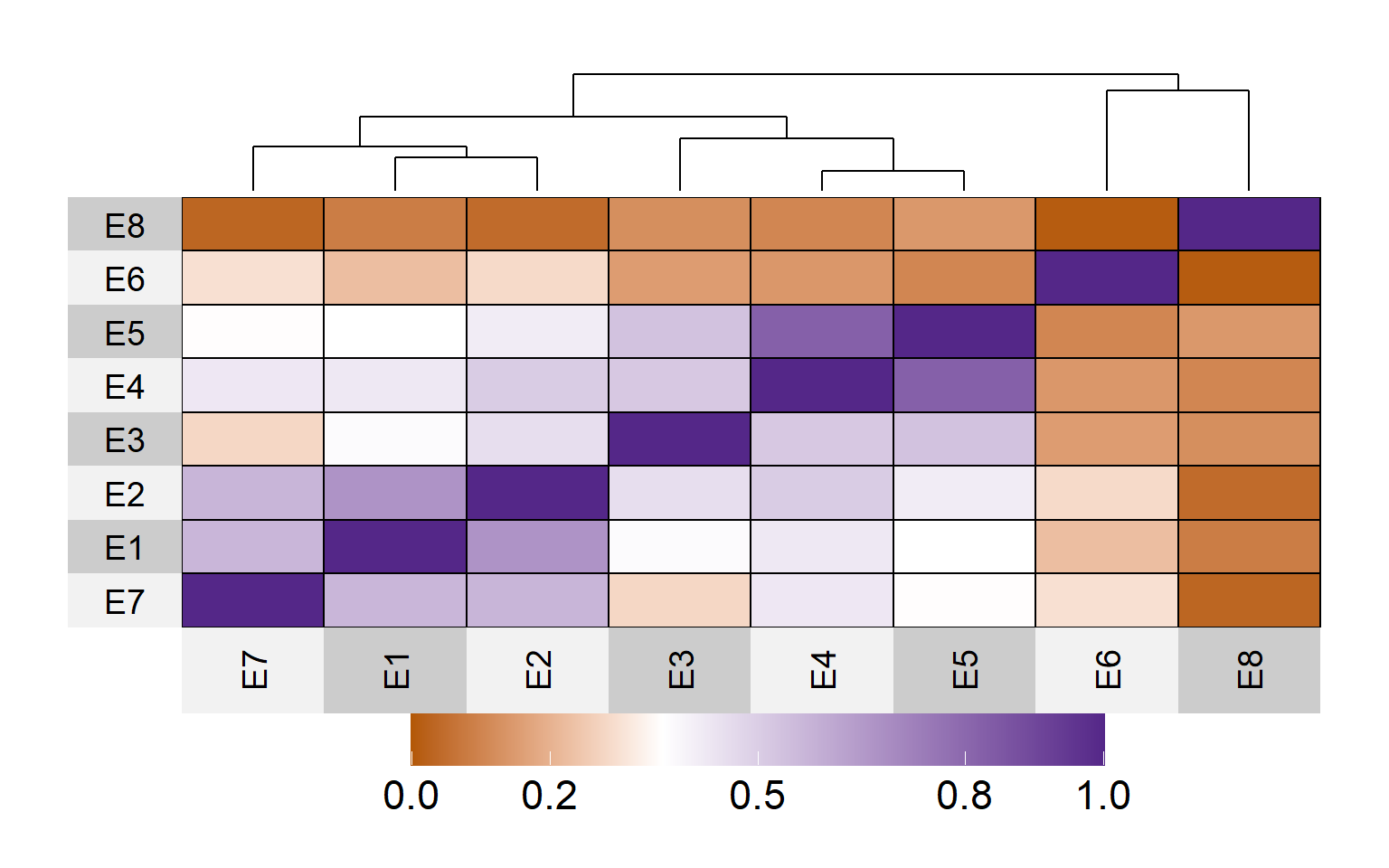
ggsave(filename = "figs/fig2_heat_env.png",
       plot = d$plot,
       width = 6,
       height = 6)
3.4 Principal Component Analysis
prec <-
  env_data %>%
  remove_cols(LON:YYYYMMDD, daysFromStart) |>
  group_by(env) %>%
  summarise(prec = sum(prec))

# compute the mean by environment and year
df_long <-
  env_data %>%
  remove_cols(LON:YYYYMMDD, daysFromStart) |>
  remove_cols(prec) %>%
  pivot_longer(-env)

# bind environment WAASB, GY, and climate traits

pca <-
  df_long %>%
  means_by(env, name) %>%
  pivot_wider(names_from = name, values_from = value) %>%
  left_join(waasb_env |> rename(GY = Y), by = "env") %>%
  left_join(prec, by = "env") %>%
  mutate(me = case_when(env %in% me1 ~ "ME1",
                        env %in% me2 ~ "ME2",
                        env %in% me3 ~ "ME3",
                        env %in% me4 ~ "ME4")) |>
  column_to_rownames("env")


# compute the PCA with
pca_model <- PCA(pca,
                 quali.sup = 17,
                 graph = FALSE)


fviz_pca_biplot(pca_model,
                repel = TRUE,
                habillage = 17,
                # font.main = c(8, "bold", "red"),
                geom.var = c("arrow", "text"),
                title = NULL) +
  my_theme +
  theme(legend.title = element_blank())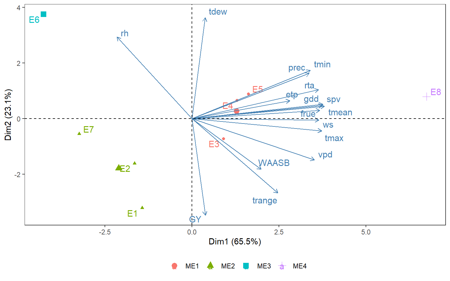
ggsave("figs/fig3_pca.png", width = 4, height = 4)3.5 Environmental tipology
names.window <-
  c('1-Tillering',
    '2-Boosting',
    '3-heading/flowering',
    '4-kernel milk stage',
    '5-physiological maturity',
    "")

out <-
  env_typing(env.data = env_data,
             env.id = "env",
             var.id = c("tmax", "vpd", "rta", "etp", "rh"),
             by.interval = TRUE,
             time.window = c(0, 30, 55, 70, 95, 130),
             names.window = names.window)

out2 <-
  separate(out,
           env.variable,
           into = c("var", "freq"),
           sep = "_",
           extra = "drop") |>
  mutate(me = case_when(env %in% me1 ~ "ME1",
                        env %in% me2 ~ "ME2",
                        env %in% me3 ~ "ME3",
                        env %in% me4 ~ "ME4"))

# plot the distribution of envirotypes
variable <- "tmax"
p1 <-
  out2 |>
  subset(var == variable) |> # change the variable here
  ggplot() +
  geom_bar(aes(x=Freq, y=env,fill=freq),
           position = "fill",
           stat = "identity",
           width = 1,
           color = "white",
           size=.2)+
  facet_grid(me~interval, scales = "free", space = "free")+
  scale_y_discrete(expand = c(0,0))+
  scale_x_continuous(expand = c(0,0))+
  xlab('Relative Frequency of the maximum air temperature (ºC)')+
  ylab("Environment")+
  labs(fill='Envirotype')+
  theme(axis.title = element_text(size=12),
        legend.text = element_text(size=9),
        strip.text = element_text(size=12),
        legend.title = element_text(size=12),
        strip.background = element_rect(fill="gray95",size=1),
        legend.position = 'bottom')

# by mega environment
p2 <-
  out2 |>
  subset(var == variable) |> # change the variable here
  sum_by(me, freq, interval) |>
  ggplot() +
  geom_bar(aes(x=Freq, y=me,fill=freq),
           position = "fill",
           stat = "identity",
           width = 1,
           color = "white",
           size=.2)+
  facet_wrap(~interval, nrow = 1)+
  scale_y_discrete(expand = c(0,0))+
  scale_x_continuous(expand = c(0,0))+
  xlab('Relative Frequency of the maximum air temperature (ºC)')+
  ylab("Mega Environment")+
  labs(fill='Envirotype')+
  theme(axis.title = element_text(size=12),
        legend.text = element_text(size=9),
        strip.text = element_text(size=12),
        legend.title = element_text(size=12),
        strip.background = element_rect(fill="gray95",size=1),
        legend.position = 'bottom') +
  scale_fill_discrete(direction = 1)

arrange_ggplot(p1, p2,
               heights = c(0.6, 0.4),
               tag_levels = "a",
               guides = "collect")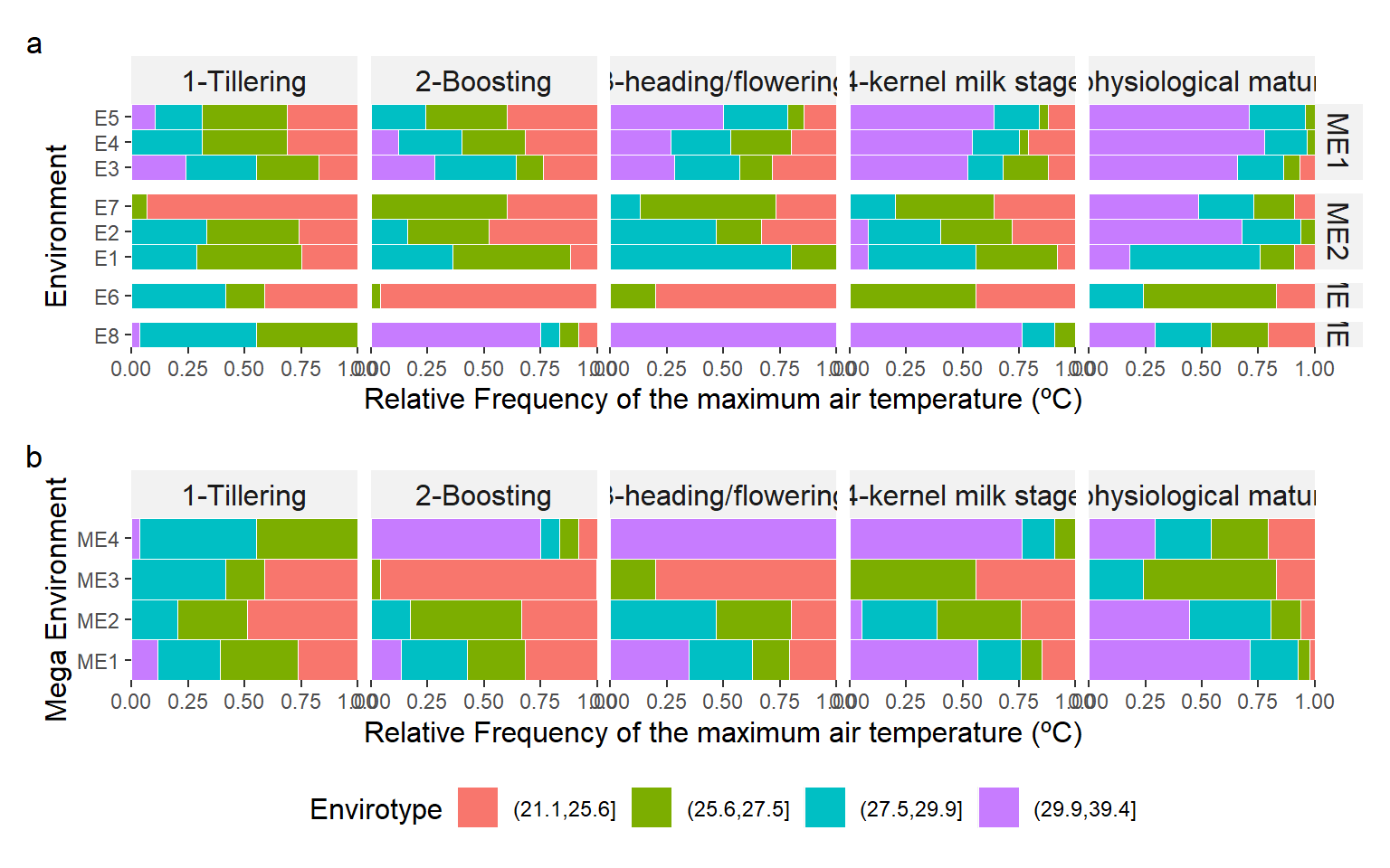
ggsave("figs/fig4_typology_tmax.png", width = 12, height = 7)4 Section info
sessionInfo()
## R version 4.2.2 (2022-10-31 ucrt)
## Platform: x86_64-w64-mingw32/x64 (64-bit)
## Running under: Windows 10 x64 (build 22621)
##
## Matrix products: default
##
## locale:
## [1] LC_COLLATE=Portuguese_Brazil.utf8  LC_CTYPE=Portuguese_Brazil.utf8
## [3] LC_MONETARY=Portuguese_Brazil.utf8 LC_NUMERIC=C
## [5] LC_TIME=Portuguese_Brazil.utf8
##
## attached base packages:
## [1] stats     graphics  grDevices utils     datasets  methods   base
##
## other attached packages:
##  [1] corrr_0.4.4       superheat_0.1.0   sp_1.5-1          ggrepel_0.9.2
##  [5] FactoMineR_2.7    factoextra_1.0.7  rio_0.5.29        metan_1.17.0.9000
##  [9] EnvRtype_1.1.0    forcats_0.5.2     stringr_1.5.0     dplyr_1.0.10
## [13] purrr_0.3.5       readr_2.1.3       tidyr_1.2.1       tibble_3.1.8
## [17] ggplot2_3.4.0     tidyverse_1.3.2
##
## loaded via a namespace (and not attached):
##   [1] readxl_1.4.1         backports_1.4.1      systemfonts_1.0.4
##   [4] plyr_1.8.8           splines_4.2.2        TH.data_1.1-1
##   [7] digest_0.6.31        foreach_1.5.2        htmltools_0.5.4
##  [10] lmerTest_3.1-3       fansi_1.0.3          magrittr_2.0.3
##  [13] googlesheets4_1.0.1  cluster_2.1.4        tzdb_0.3.0
##  [16] openxlsx_4.2.5.1     modelr_0.1.10        sandwich_3.0-2
##  [19] svglite_2.1.0        timechange_0.1.1     rmdformats_1.0.4
##  [22] colorspace_2.0-3     rvest_1.0.3          textshaping_0.3.6
##  [25] haven_2.5.1          xfun_0.35            crayon_1.5.2
##  [28] jsonlite_1.8.4       lme4_1.1-31          survival_3.4-0
##  [31] zoo_1.8-11           iterators_1.0.14     glue_1.6.2
##  [34] kableExtra_1.3.4     polyclip_1.10-4      gtable_0.3.1
##  [37] gargle_1.2.1         emmeans_1.8.3        webshot_0.5.4
##  [40] car_3.1-1            abind_1.4-5          scales_1.2.1
##  [43] mvtnorm_1.1-3        DBI_1.1.3            GGally_2.1.2
##  [46] rstatix_0.7.1        Rcpp_1.0.9           viridisLite_0.4.1
##  [49] xtable_1.8-4         flashClust_1.01-2    foreign_0.8-83
##  [52] DT_0.26              htmlwidgets_1.6.0    httr_1.4.4
##  [55] RColorBrewer_1.1-3   ellipsis_0.3.2       pkgconfig_2.0.3
##  [58] reshape_0.8.9        farver_2.1.1         multcompView_0.1-8
##  [61] sass_0.4.4           dbplyr_2.2.1         utf8_1.2.2
##  [64] tidyselect_1.2.0     labeling_0.4.2       rlang_1.0.6
##  [67] reshape2_1.4.4       munsell_0.5.0        cellranger_1.1.0
##  [70] tools_4.2.2          cachem_1.0.6         cli_3.4.1
##  [73] generics_0.1.3       broom_1.0.2          mathjaxr_1.6-0
##  [76] evaluate_0.19        fastmap_1.1.0        ggdendro_0.1.23
##  [79] yaml_2.3.6           ragg_1.2.4           knitr_1.41
##  [82] fs_1.5.2             zip_2.2.2            nlme_3.1-160
##  [85] leaps_3.1            xml2_1.3.3           compiler_4.2.2
##  [88] rstudioapi_0.14      curl_4.3.3           ggsignif_0.6.4
##  [91] reprex_2.0.2         tweenr_2.0.2         bslib_0.4.2
##  [94] stringi_1.7.8        highr_0.9            lattice_0.20-45
##  [97] Matrix_1.5-3         nloptr_2.0.3         vctrs_0.5.1
## [100] pillar_1.8.1         lifecycle_1.0.3      jquerylib_0.1.4
## [103] estimability_1.4.1   data.table_1.14.6    patchwork_1.1.2
## [106] R6_2.5.1             bookdown_0.31        codetools_0.2-18
## [109] boot_1.3-28          MASS_7.3-58.1        assertthat_0.2.1
## [112] withr_2.5.0          multcomp_1.4-20      hms_1.1.2
## [115] grid_4.2.2           coda_0.19-4          minqa_1.2.5
## [118] rmarkdown_2.19       carData_3.0-5        googledrive_2.0.0
## [121] ggpubr_0.5.0         ggforce_0.4.1        numDeriv_2016.8-1.1
## [124] scatterplot3d_0.3-42 lubridate_1.9.0