Analysis
1 Libraries
To reproduce the examples of this material, the R packages the following packages are needed.
# it is suggested to use the dev version of metan package
# remotes::install_github("TiagoOlivoto/metan")

library(EnvRtype)
library(rio)
library(factoextra)
library(FactoMineR)
library(ggrepel)
library(ggh4x)
library(superheat)
library(ggridges)
library(metan)
library(rnaturalearth)
library(lme4)
library(lmerTest)
library(broom.mixed)
library(tidyverse)
library(ggsn)

# a ggplot2 theme for the plots
my_theme <-
  theme_bw() +
  theme(panel.spacing = unit(0, "cm"),
        panel.grid = element_blank(),
        legend.position = "bottom")
2 Dataset
df_traits <-
  import("data/df_traits.csv") |>
  metan::as_factor(1:6)


# long data
df_traits_long <-
  df_traits |>
  pivot_longer(GMC:HSW)


# grain yield mean in each environment
df_gy <-
  df_traits |>
  mean_by(ME, YEAR, .vars = GY)

# genotypic variance in each mega-environment
df_var_gy <-
  df_traits |>
  group_by(YEAR, ME) |>
  do(lmer(GY ~(1|GEN), data = .) |>
       tidy(effects = "ran_pars") |>
       filter(group == "GEN") |>
       transmute(var = estimate^2))
3 Location map
china <-
  ne_states(country = c("china", "taiwan"),
            returnclass = "sf")

locs <-
  import("https://bit.ly/local_info") %>%
  distinct(Lat, .keep_all = TRUE)

china <-
  mutate(china,
         Province = ifelse(name %in% locs$Province, name, NA))

png("figs/fig1_map1.jpeg", width = 10, height = 7, units = "in", res = 600)

ggplot(data = china) +
  geom_sf(aes(fill = Province), size = 0.2) +
  ggthemes::theme_map() +
  scale_fill_discrete(na.value = "gray97",
                      labels = c(unique(locs$Province), "others")) +
  theme(legend.position = "none")
dev.off()
## png
##   2


png("figs/fig1_map2.jpeg", width = 10, height = 7, units = "in", res = 600)

zoom <-
  ggplot(data = china) +
  geom_sf(aes(fill = Province), size = 0.2) +
  ggthemes::theme_map() +
  scale_fill_discrete(na.value = "gray97",
                      labels = c(unique(locs$Province), "others")) +
  geom_point(data = locs,
             aes(x = Lon, y = Lat, size = Altitude),
             color = "black",
             fill = "red",
             shape = 21) +
  geom_label_repel(data = locs,
                   aes(label = Location,
                       x = Lon,
                       y = Lat),
                   fill = "green",
                   color = "black",
                   segment.color = 'black',
                   force = 38,
                   size = 4) +
  theme(legend.position = c(0.95, 0.1)) +
  theme_minimal() +
  theme(legend.position = c(.95, 0.55)) +
  scalebar(dist = 200,
           x.min = 109,
           x.max = 128,
           y.min = 29.5,
           y.max = 42,
           dist_unit = "km",
           transform = TRUE,
           model = "WGS84") +
  xlim(c(109, 128)) +
  ylim(c(28, 42)) +
  labs(x = "Longitude",
       y = "Latitude")


north2(zoom, 0.9, .1)
dev.off()
## png
##   2
4 Mega-environment delineation
4.1 20-year climate data
df_years <- import("data/me_delineation.csv")
ENV <- df_years$Code
LAT <- df_years$Lat
LON <- df_years$Lon
ALT <- df_years$Alt
START <- df_years$Sowing
END <- df_years$Harvesting

# see more at https://github.com/allogamous/EnvRtype
df_climate <-
  get_weather(env.id = ENV,
              lat = LAT,
              lon = LON,
              start.day = START,
              end.day = END,
              parallel = TRUE)

# GDD: Growing Degree Day (oC/day)
# FRUE: Effect of temperature on radiation use efficiency (from 0 to 1)
# T2M_RANGE: Daily Temperature Range (oC day)
# SPV: Slope of saturation vapour pressure curve (kPa.Celsius)
# VPD: Vapour pressure deficit (kPa)
# ETP: Potential Evapotranspiration (mm.day)
# PEPT: Deficit by Precipitation (mm.day)
# n: Actual duration of sunshine (hour)
# N: Daylight hours (hour)


# RTA: Extraterrestrial radiation (MJ/m^2/day)
# T2M: Temperature at 2 Meters
# T2M_MAX: Maximum Temperature at 2 Meters
# T2M_MIN: Minimum Temperature at 2 Meters
# PRECTOT: Precipitation
# WS2M: Wind Speed at 2 Meters
# RH2M: Relative Humidity at 2 Meters
# T2MDEW: Dew/Frost Point at 2 Meters
# ALLSKY_SFC_LW_DWN: Downward Thermal Infrared (Longwave) Radiative Flux
# ALLSKY_SFC_SW_DWN: All Sky Insolation Incident on a Horizontal Surface
# ALLSKY_TOA_SW_DWN: Top-of-atmosphere Insolation
# [1] "env"       "ETP"       "GDD"         "PETP"      "RH2M"      "SPV"
# [8] "T2M"       "T2M_MAX"   "T2M_MIN"   "T2M_RANGE" "T2MDEW"    "VPD"

# Compute other parameters
env_data <-
  df_climate %>%
  as.data.frame() %>%
  param_temperature(Tbase1 = 10, # choose the base temperature here
                    Tbase2 = 33, # choose the base temperature here
                    merge = TRUE) %>%
  param_atmospheric(merge = TRUE) %>%
  param_radiation(merge = TRUE) |>
  separate(env, into = c("env", "year"), sep = "_") |>
  rename(TMAX = T2M_MAX,
         TMIN = T2M_MIN,
         ASKLW = ALLSKY_SFC_LW_DWN,
         ASKSW = ALLSKY_SFC_SW_DWN,
         TRANGE = T2M_RANGE)
env_data <- readRDS("data/env_data.Rdata")
info <-
env_data |>
dplyr::select(env, LON, LAT) |>
mean_by(env)
df_gy_loc <-
df_traits |>
mean_by(LOC, .vars = GY)
env_wider <-
env_data |>
select(env, year, daysFromStart, TMED:RTA) |>
pivot_wider(names_from = "year",
values_from = TMED:RTA) |>
left_join(info) |>
relocate(LON, LAT, .after = env) |>
mutate(MM = 1,
DD = 1,
DOY = 1,
YYYYMMDD = 1,
YEAR = 1,
.after = env)
saveRDS(env_wider, "data/env_wider.Rdata")4.2 Environmental kinships
id_var <- names(env_wider)[10:ncol(env_wider)]

EC <-
  W_matrix(env.data = env_wider,
           env.id = "env",
           var.id = id_var,
           by.interval = TRUE,
           time.window = c(0, 30, 60, 90, 120, 150),
           QC = TRUE,
           sd.tol = 3)
## ------------------------------------------------
## Quality Control based on sd.tol=3
## Removed variables:
## 271 from 2280
## DTIRF_2001_mean_Interval_0
##  DTIRF_2001_mean_Interval_30
##  DTIRF_2001_mean_Interval_60
##  DTIRF_2001_mean_Interval_90
##  DTIRF_2001_mean_Interval_120
##  DTIRF_2001_mean_Interval_150
##  DTIRF_2002_mean_Interval_0
##  DTIRF_2002_mean_Interval_30
##  DTIRF_2002_mean_Interval_60
##  DTIRF_2002_mean_Interval_90
##  DTIRF_2002_mean_Interval_120
##  DTIRF_2002_mean_Interval_150
##  DTIRF_2003_mean_Interval_0
##  DTIRF_2003_mean_Interval_30
##  DTIRF_2003_mean_Interval_60
##  DTIRF_2003_mean_Interval_90
##  DTIRF_2003_mean_Interval_120
##  DTIRF_2003_mean_Interval_150
##  DTIRF_2004_mean_Interval_0
##  DTIRF_2004_mean_Interval_30
##  DTIRF_2004_mean_Interval_60
##  DTIRF_2004_mean_Interval_90
##  DTIRF_2004_mean_Interval_120
##  DTIRF_2004_mean_Interval_150
##  DTIRF_2005_mean_Interval_0
##  DTIRF_2005_mean_Interval_30
##  DTIRF_2005_mean_Interval_60
##  DTIRF_2005_mean_Interval_90
##  DTIRF_2005_mean_Interval_120
##  DTIRF_2005_mean_Interval_150
##  DTIRF_2006_mean_Interval_0
##  DTIRF_2006_mean_Interval_30
##  DTIRF_2006_mean_Interval_60
##  DTIRF_2006_mean_Interval_90
##  DTIRF_2006_mean_Interval_120
##  DTIRF_2006_mean_Interval_150
##  DTIRF_2007_mean_Interval_0
##  DTIRF_2007_mean_Interval_30
##  DTIRF_2007_mean_Interval_60
##  DTIRF_2007_mean_Interval_90
##  DTIRF_2007_mean_Interval_120
##  DTIRF_2007_mean_Interval_150
##  DTIRF_2008_mean_Interval_0
##  DTIRF_2008_mean_Interval_30
##  DTIRF_2008_mean_Interval_60
##  DTIRF_2008_mean_Interval_90
##  DTIRF_2008_mean_Interval_120
##  DTIRF_2008_mean_Interval_150
##  DTIRF_2009_mean_Interval_0
##  DTIRF_2009_mean_Interval_30
##  DTIRF_2009_mean_Interval_60
##  DTIRF_2009_mean_Interval_90
##  DTIRF_2009_mean_Interval_120
##  DTIRF_2009_mean_Interval_150
##  DTIRF_2010_mean_Interval_0
##  DTIRF_2010_mean_Interval_30
##  DTIRF_2010_mean_Interval_60
##  DTIRF_2010_mean_Interval_90
##  DTIRF_2010_mean_Interval_120
##  DTIRF_2010_mean_Interval_150
##  DTIRF_2011_mean_Interval_0
##  DTIRF_2011_mean_Interval_30
##  DTIRF_2011_mean_Interval_60
##  DTIRF_2011_mean_Interval_90
##  DTIRF_2011_mean_Interval_120
##  DTIRF_2011_mean_Interval_150
##  DTIRF_2012_mean_Interval_0
##  DTIRF_2012_mean_Interval_30
##  DTIRF_2012_mean_Interval_60
##  DTIRF_2012_mean_Interval_90
##  DTIRF_2012_mean_Interval_120
##  DTIRF_2012_mean_Interval_150
##  DTIRF_2013_mean_Interval_0
##  DTIRF_2013_mean_Interval_30
##  DTIRF_2013_mean_Interval_60
##  DTIRF_2013_mean_Interval_90
##  DTIRF_2013_mean_Interval_120
##  DTIRF_2013_mean_Interval_150
##  DTIRF_2014_mean_Interval_0
##  DTIRF_2014_mean_Interval_30
##  DTIRF_2014_mean_Interval_60
##  DTIRF_2014_mean_Interval_90
##  DTIRF_2014_mean_Interval_120
##  DTIRF_2014_mean_Interval_150
##  DTIRF_2015_mean_Interval_0
##  DTIRF_2015_mean_Interval_30
##  DTIRF_2015_mean_Interval_60
##  DTIRF_2015_mean_Interval_90
##  DTIRF_2015_mean_Interval_120
##  DTIRF_2015_mean_Interval_150
##  DTIRF_2016_mean_Interval_0
##  DTIRF_2016_mean_Interval_30
##  DTIRF_2016_mean_Interval_60
##  DTIRF_2016_mean_Interval_90
##  DTIRF_2016_mean_Interval_120
##  DTIRF_2016_mean_Interval_150
##  DTIRF_2017_mean_Interval_0
##  DTIRF_2017_mean_Interval_30
##  DTIRF_2017_mean_Interval_60
##  DTIRF_2017_mean_Interval_90
##  DTIRF_2017_mean_Interval_120
##  DTIRF_2017_mean_Interval_150
##  DTIRF_2018_mean_Interval_0
##  DTIRF_2018_mean_Interval_30
##  DTIRF_2018_mean_Interval_60
##  DTIRF_2018_mean_Interval_90
##  DTIRF_2018_mean_Interval_120
##  DTIRF_2018_mean_Interval_150
##  DTIRF_2019_mean_Interval_0
##  DTIRF_2019_mean_Interval_30
##  DTIRF_2019_mean_Interval_60
##  DTIRF_2019_mean_Interval_90
##  DTIRF_2019_mean_Interval_120
##  DTIRF_2019_mean_Interval_150
##  DTIRF_2020_mean_Interval_0
##  DTIRF_2020_mean_Interval_30
##  DTIRF_2020_mean_Interval_60
##  DTIRF_2020_mean_Interval_90
##  DTIRF_2020_mean_Interval_120
##  DTIRF_2020_mean_Interval_150
##  PETP_2002_mean_Interval_0
##  PETP_2003_mean_Interval_60
##  PETP_2005_mean_Interval_60
##  PETP_2006_mean_Interval_60
##  PETP_2007_mean_Interval_60
##  PETP_2010_mean_Interval_90
##  PETP_2013_mean_Interval_60
##  PETP_2015_mean_Interval_30
##  PETP_2017_mean_Interval_120
##  PETP_2018_mean_Interval_0
##  PETP_2018_mean_Interval_90
##  PETP_2019_mean_Interval_90
##  PETP_2020_mean_Interval_30
##  PETP_2020_mean_Interval_60
##  PETP_2020_mean_Interval_90
##  PRECTOT_2003_mean_Interval_60
##  PRECTOT_2005_mean_Interval_60
##  PRECTOT_2007_mean_Interval_60
##  PRECTOT_2017_mean_Interval_120
##  PRECTOT_2020_mean_Interval_30
##  PRECTOT_2020_mean_Interval_60
##  RH_2001_mean_Interval_0
##  RH_2001_mean_Interval_30
##  RH_2001_mean_Interval_60
##  RH_2001_mean_Interval_90
##  RH_2001_mean_Interval_120
##  RH_2001_mean_Interval_150
##  RH_2002_mean_Interval_0
##  RH_2002_mean_Interval_30
##  RH_2002_mean_Interval_60
##  RH_2002_mean_Interval_90
##  RH_2002_mean_Interval_120
##  RH_2002_mean_Interval_150
##  RH_2003_mean_Interval_0
##  RH_2003_mean_Interval_30
##  RH_2003_mean_Interval_60
##  RH_2003_mean_Interval_90
##  RH_2003_mean_Interval_120
##  RH_2003_mean_Interval_150
##  RH_2004_mean_Interval_0
##  RH_2004_mean_Interval_30
##  RH_2004_mean_Interval_60
##  RH_2004_mean_Interval_90
##  RH_2004_mean_Interval_120
##  RH_2004_mean_Interval_150
##  RH_2005_mean_Interval_0
##  RH_2005_mean_Interval_30
##  RH_2005_mean_Interval_60
##  RH_2005_mean_Interval_90
##  RH_2005_mean_Interval_120
##  RH_2005_mean_Interval_150
##  RH_2006_mean_Interval_0
##  RH_2006_mean_Interval_30
##  RH_2006_mean_Interval_60
##  RH_2006_mean_Interval_90
##  RH_2006_mean_Interval_120
##  RH_2006_mean_Interval_150
##  RH_2007_mean_Interval_0
##  RH_2007_mean_Interval_30
##  RH_2007_mean_Interval_60
##  RH_2007_mean_Interval_90
##  RH_2007_mean_Interval_120
##  RH_2007_mean_Interval_150
##  RH_2008_mean_Interval_0
##  RH_2008_mean_Interval_30
##  RH_2008_mean_Interval_60
##  RH_2008_mean_Interval_90
##  RH_2008_mean_Interval_120
##  RH_2008_mean_Interval_150
##  RH_2009_mean_Interval_0
##  RH_2009_mean_Interval_30
##  RH_2009_mean_Interval_60
##  RH_2009_mean_Interval_90
##  RH_2009_mean_Interval_150
##  RH_2010_mean_Interval_0
##  RH_2010_mean_Interval_30
##  RH_2010_mean_Interval_60
##  RH_2010_mean_Interval_90
##  RH_2010_mean_Interval_150
##  RH_2011_mean_Interval_0
##  RH_2011_mean_Interval_30
##  RH_2011_mean_Interval_60
##  RH_2011_mean_Interval_90
##  RH_2011_mean_Interval_150
##  RH_2012_mean_Interval_0
##  RH_2012_mean_Interval_30
##  RH_2012_mean_Interval_60
##  RH_2012_mean_Interval_90
##  RH_2012_mean_Interval_150
##  RH_2013_mean_Interval_0
##  RH_2013_mean_Interval_30
##  RH_2013_mean_Interval_60
##  RH_2013_mean_Interval_90
##  RH_2013_mean_Interval_120
##  RH_2013_mean_Interval_150
##  RH_2014_mean_Interval_0
##  RH_2014_mean_Interval_30
##  RH_2014_mean_Interval_60
##  RH_2014_mean_Interval_90
##  RH_2014_mean_Interval_120
##  RH_2014_mean_Interval_150
##  RH_2015_mean_Interval_0
##  RH_2015_mean_Interval_30
##  RH_2015_mean_Interval_60
##  RH_2015_mean_Interval_90
##  RH_2015_mean_Interval_120
##  RH_2015_mean_Interval_150
##  RH_2016_mean_Interval_0
##  RH_2016_mean_Interval_30
##  RH_2016_mean_Interval_60
##  RH_2016_mean_Interval_90
##  RH_2016_mean_Interval_120
##  RH_2016_mean_Interval_150
##  RH_2017_mean_Interval_0
##  RH_2017_mean_Interval_30
##  RH_2017_mean_Interval_60
##  RH_2017_mean_Interval_90
##  RH_2017_mean_Interval_120
##  RH_2017_mean_Interval_150
##  RH_2018_mean_Interval_0
##  RH_2018_mean_Interval_30
##  RH_2018_mean_Interval_60
##  RH_2018_mean_Interval_90
##  RH_2018_mean_Interval_120
##  RH_2018_mean_Interval_150
##  RH_2019_mean_Interval_0
##  RH_2019_mean_Interval_30
##  RH_2019_mean_Interval_60
##  RH_2019_mean_Interval_90
##  RH_2019_mean_Interval_120
##  RH_2019_mean_Interval_150
##  RH_2020_mean_Interval_0
##  RH_2020_mean_Interval_30
##  RH_2020_mean_Interval_60
##  RH_2020_mean_Interval_90
##  RH_2020_mean_Interval_120
##  RH_2020_mean_Interval_150
##  SIHS_2014_mean_Interval_0
##  SIHS_2019_mean_Interval_0
##  T2MDEW_2001_mean_Interval_0
##  T2MDEW_2002_mean_Interval_150
##  T2MDEW_2005_mean_Interval_0
##  T2MDEW_2006_mean_Interval_0
##  T2MDEW_2007_mean_Interval_0
##  T2MDEW_2009_mean_Interval_30
##  T2MDEW_2013_mean_Interval_0
##  T2MDEW_2014_mean_Interval_0
##  T2MDEW_2015_mean_Interval_0
##  T2MDEW_2016_mean_Interval_0
##  T2MDEW_2017_mean_Interval_0
##  T2MDEW_2019_mean_Interval_0
## ------------------------------------------------

saveRDS(EC, "data/EC.Rdata")
4.3 Heatmap
distances <-
  env_kernel(env.data = EC,
             gaussian = TRUE)
d <-
  superheat(distances[[2]],
            heat.pal = c("#b35806", "white", "#542788"),
            pretty.order.rows = TRUE,
            pretty.order.cols = TRUE,
            col.dendrogram = TRUE,
            legend.width = 4,
            left.label.size = 0.1,
            bottom.label.text.size = 5,
            bottom.label.size = 0.2,
            bottom.label.text.angle = 90,
            legend.text.size = 17,
            heat.lim = c(0, 1),
            padding = 0.5,
            legend.height=0.2)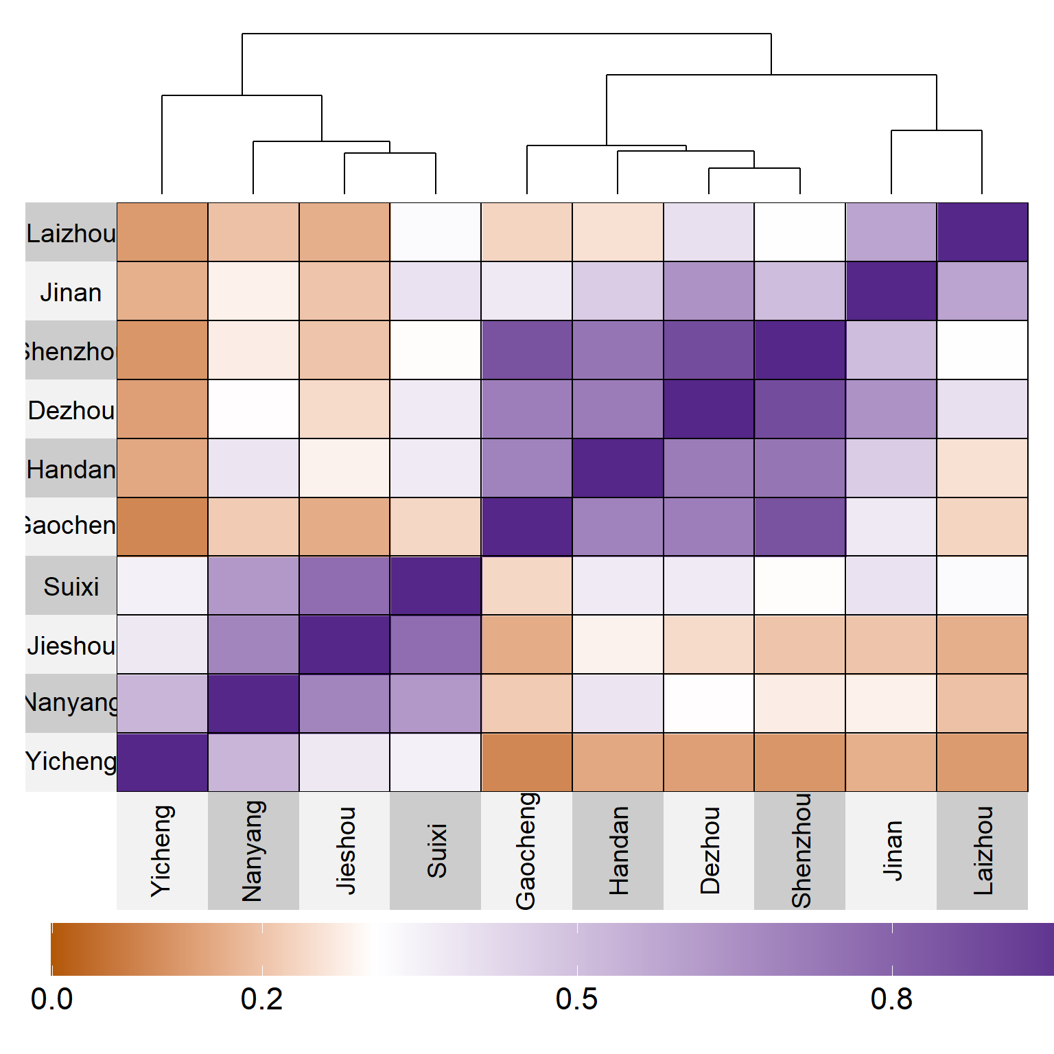
Figure 4.1: Similarity
ggsave(filename = "figs/fig2_heat_env2.pdf",
       plot = d$plot,
       width = 11,
       height = 10)


env_data <-
  env_data |>
  mutate(me = case_when(
    env %in% c("Yicheng") ~ "ME1",
    env %in% c("Suixi", "Jieshou", "Nanyang") ~ "ME2",
    env %in% c("Shenzhou", "Gaocheng", "Handan", "Dezhou") ~ "ME3",
    env %in% c("Laizhou", "Jinan") ~ "ME4"
  ),
  .after = env)
4.4 Principal component analysis
env_data_m <-
  env_data |>
  select(-daysFromStart) |>
  mean_by(me, .vars = TMED:RTA) |>
  column_to_rownames("me")

# compute the PCA with
pca_model_h <- PCA(env_data_m,
                   graph = FALSE)

bp1 <-
  fviz_pca_biplot(pca_model_h,
                  repel = TRUE,
                  col.var = "steelblue",
                  title = NULL) +
  coord_equal() +
  labs(title = "Long-term weather (20 years)")
5 Climate variables (trials)
5.1 Getting the data
df_env <- import("data/location_info.csv")
ENV <- df_env$Code
LAT <- df_env$Lat
LON <- df_env$Lon
ALT <- df_env$Alt
START <- df_env$Sowing
END <- df_env$Harvesting

# see more at https://github.com/allogamous/EnvRtype
df_climate <-
  get_weather(env.id = ENV,
              lat = LAT,
              lon = LON,
              start.day = START,
              end.day = END)
# GDD: Growing Degree Day (oC/day)
# FRUE: Effect of temperature on radiation use efficiency (from 0 to 1)
# T2M_RANGE: Daily Temperature Range (oC day)
# SPV: Slope of saturation vapour pressure curve (kPa.Celsius)
# VPD: Vapour pressure deficit (kPa)
# ETP: Potential Evapotranspiration (mm.day)
# PEPT: Deficit by Precipitation (mm.day)
# n: Actual duration of sunshine (hour)
# N: Daylight hours (hour)
# RTA: Extraterrestrial radiation (MJ/m^2/day)
# SRAD: Solar radiation (MJ/m^2/day)
# T2M: Temperature at 2 Meters
# T2M_MAX: Maximum Temperature at 2 Meters
# T2M_MIN: Minimum Temperature at 2 Meters
# PRECTOT: Precipitation
# WS2M: Wind Speed at 2 Meters
# RH2M: Relative Humidity at 2 Meters
# T2MDEW: Dew/Frost Point at 2 Meters
# ALLSKY_SFC_LW_DWN: Downward Thermal Infrared (Longwave) Radiative Flux
# ALLSKY_SFC_SW_DWN: All Sky Insolation Incident on a Horizontal Surface
# ALLSKY_TOA_SW_DWN: Top-of-atmosphere Insolation
# [1] "env"       "ETP"       "GDD"         "PETP"      "RH2M"      "SPV"
# [8] "T2M"       "T2M_MAX"   "T2M_MIN"   "T2M_RANGE" "T2MDEW"    "VPD"

# Compute other parameters
env_data <-
  df_climate %>%
  as.data.frame() %>%
  param_temperature(Tbase1 = 10, # choose the base temperature here
                    Tbase2 = 33, # choose the base temperature here
                    merge = TRUE) %>%
  param_atmospheric(merge = TRUE) %>%
  param_radiation(merge = TRUE) |>
  rename(DTIRF = ALLSKY_SFC_LW_DWN,
         SIHS = ALLSKY_SFC_SW_DWN,
         TMIN = T2M_MIN,
         TMAX = T2M_MAX,
         TMED = T2M,
         RH = RH2M,
         WS = WS2M,
         TRANGE = T2M_RANGE) |>
  separate(env, into = c("ENV", "YEAR")) |>
  relocate(daysFromStart, .before = TMED) |>
  mutate(ME = case_when(
    ENV %in% c("Yicheng") ~ "ME1",
    ENV %in% c("Suixi", "Jieshou", "Nanyang") ~ "ME2",
    ENV %in% c("Shenzhou", "Gaocheng", "Handan", "Dezhou") ~ "ME3",
    ENV %in% c("Laizhou", "Jinan") ~ "ME4"
  ),
  .after = ENV)

export(env_data, "data/env_data_trial.xlsx")
5.2 Tidy climate data
env_data_trial <- import("data/env_data_trial.xlsx")5.3 Principal component analysis
names_var <- names(env_data_trial)[11:ncol(env_data_trial)]


pca_2019 <-
  env_data_trial |>
  mean_by(ME, YEAR, .vars = names_var) |>
  metan::as_factor(1:2) |>
  left_join(df_gy) |>
  left_join(df_var_gy) |>
  filter(YEAR == 2019) |>
  left_join(df_gy) |>
  left_join(df_var_gy) |>
  remove_cols(YEAR) |>
  column_to_rownames("ME")

pca_2020 <-
  env_data_trial |>
  mean_by(ME, YEAR, .vars = names_var) |>
  metan::as_factor(1:2) |>
  left_join(df_gy) |>
  left_join(df_var_gy) |>
  filter(YEAR == 2020) |>
  left_join(df_gy) |>
  left_join(df_var_gy) |>
  remove_cols(YEAR) |>
  column_to_rownames("ME")


pca2 <-
  env_data_trial |>
  mean_by(ME, .vars = names_var) |>
  left_join(df_gy |> mean_by(ME)) |>
  left_join(df_var_gy|> mean_by(ME)) |>
  column_to_rownames("ME")


# compute the PCA with

pca2019 <- PCA(pca_2019, graph = FALSE)
pca2020 <- PCA(pca_2020, graph = FALSE)
pca_model2 <- PCA(pca2,  graph = FALSE)


bip1 <-
  fviz_pca_biplot(pca2019,
                  repel = TRUE,
                  col.var = "steelblue",
                  title = NULL) +
  coord_equal() +
  labs(title = "Data for 2019 trials")

bip2 <-
  fviz_pca_biplot(pca2020,
                  repel = TRUE,
                  col.var = "steelblue",
                  title = NULL) +
  coord_equal() +
  labs(title = "Data for 2020 trials")


bip3 <-
  fviz_pca_biplot(pca_model2,
                  repel = TRUE,
                  col.var = "steelblue",
                  title = NULL) +
  coord_equal() +
  labs(title = "Average data")


arrange_ggplot(bp1, bip1, bip2, bip3,
               tag_levels = "A")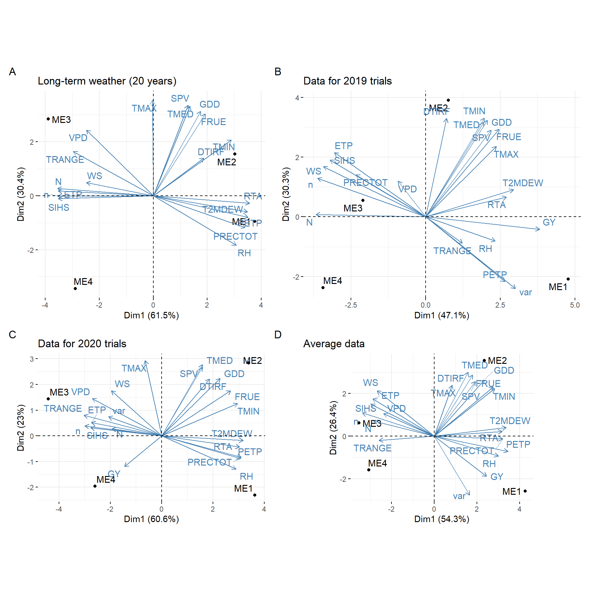
Figure 5.1: biplot for PCA
ggsave("figs/fig3_pca.jpeg", width = 11, height = 11)5.4 Environmental tipology (vapor pressure deficit)
names.window <- c('1-intial growing','2-leaf expansion I','3-leaf expansion II','4-flowering','5-grain filling', "")


out <-
  env_data_trial |>
  concatenate(ME, YEAR, .after = YEAR, new_var = env) |>
  env_typing(env.id = c("YEAR, ME"),
             var.id = names_var,
             by.interval = TRUE,
             time.window = c(0, 15, 35, 65, 90, 120),
             names.window = names.window,
             quantiles = c(.01, .25, .50, .75, .975, .99)) |>
  separate(env, into = c("ME", "YEAR")) |>
  separate(env.variable,
           into = c("var", "freq"),
           sep = "_",
           extra = "drop")
# plot the distribution of envirotypes for dbp
variable <- "VPD"
p1 <-
out |>
subset(var == variable) |> # change the variable here
# mutate()
ggplot() +
geom_bar(aes(x=Freq, y=ME,fill=freq),
position = "fill",
stat = "identity",
width = 1,
color = "white",
size=.2)+
facet_grid(YEAR~interval, scales = "free", space = "free")+
scale_y_discrete(expand = c(0,0))+
scale_x_continuous(expand = c(0,0))+
labs(x = 'Relative frequency for vapor pressure deficit',
y = "Mega-Environment",
fill='Envirotype')+
theme(axis.title = element_text(size=12),
legend.text = element_text(size=9),
strip.text = element_text(size=12),
legend.title = element_text(size=12),
strip.background = element_rect(fill="gray95",size=1)) +
ggthemes::scale_fill_stata()
# plot the distribution of envirotypes for dbp
variable <- "PETP"
p2 <-
out |>
subset(var == variable) |> # change the variable here
mutate(freq = as_factor(freq),
freq = fct_relevel(freq, "(-13.1,-9.95]", "(-9.95,-7.54]",
"(-7.54,-2.13]", "(-2.13,31.5]",
"(31.5,47.8]" )) |>
ggplot() +
geom_bar(aes(x=Freq, y=ME,fill=freq),
position = "fill",
stat = "identity",
width = 1,
color = "white",
size=.2) +
facet_grid(YEAR~interval) +
scale_y_discrete(expand = c(0,0))+
scale_x_continuous(expand = c(0,0))+
labs(x = 'Relative frequency for deficit by precipitation',
y = "Mega-Environment",
fill='Envirotype')+
theme(axis.title = element_text(size=12),
legend.text = element_text(size=9),
strip.text = element_text(size=12),
legend.title = element_text(size=12),
strip.background = element_rect(fill="gray95",size=1)) +
ggthemes::scale_fill_stata()
# plot the distribution of envirotypes for dbp
variable <- "TMIN"
p3 <-
out |>
subset(var == variable) |> # change the variable here
# mutate()
ggplot() +
geom_bar(aes(x=Freq, y=ME,fill=freq),
position = "fill",
stat = "identity",
width = 1,
color = "white",
size=.2) +
facet_grid(YEAR~interval) +
scale_y_discrete(expand = c(0,0))+
scale_x_continuous(expand = c(0,0))+
labs(x = 'Relative frequency',
y = "Mega-Environment",
fill='Envirotype')+
theme(axis.title = element_text(size=12),
legend.text = element_text(size=9),
strip.text = element_text(size=12),
legend.title = element_text(size=12),
strip.background = element_rect(fill="gray95",size=1)) +
ggthemes::scale_fill_stata()
# plot the distribution of envirotypes for dbp
variable <- "TMAX"
p4 <-
out |>
subset(var == variable) |> # change the variable here
# mutate()
ggplot() +
geom_bar(aes(x=Freq, y=ME,fill=freq),
position = "fill",
stat = "identity",
width = 1,
color = "white",
size=.2) +
facet_grid(YEAR~interval) +
scale_y_discrete(expand = c(0,0))+
scale_x_continuous(expand = c(0,0))+
labs(x = 'Relative frequency',
y = "Mega-Environment",
fill='Envirotype')+
theme(axis.title = element_text(size=12),
legend.text = element_text(size=9),
strip.text = element_text(size=12),
legend.title = element_text(size=12),
strip.background = element_rect(fill="gray95",size=1)) +
ggthemes::scale_fill_stata()
arrange_ggplot(p1, p2,
ncol = 1,
tag_levels = "A")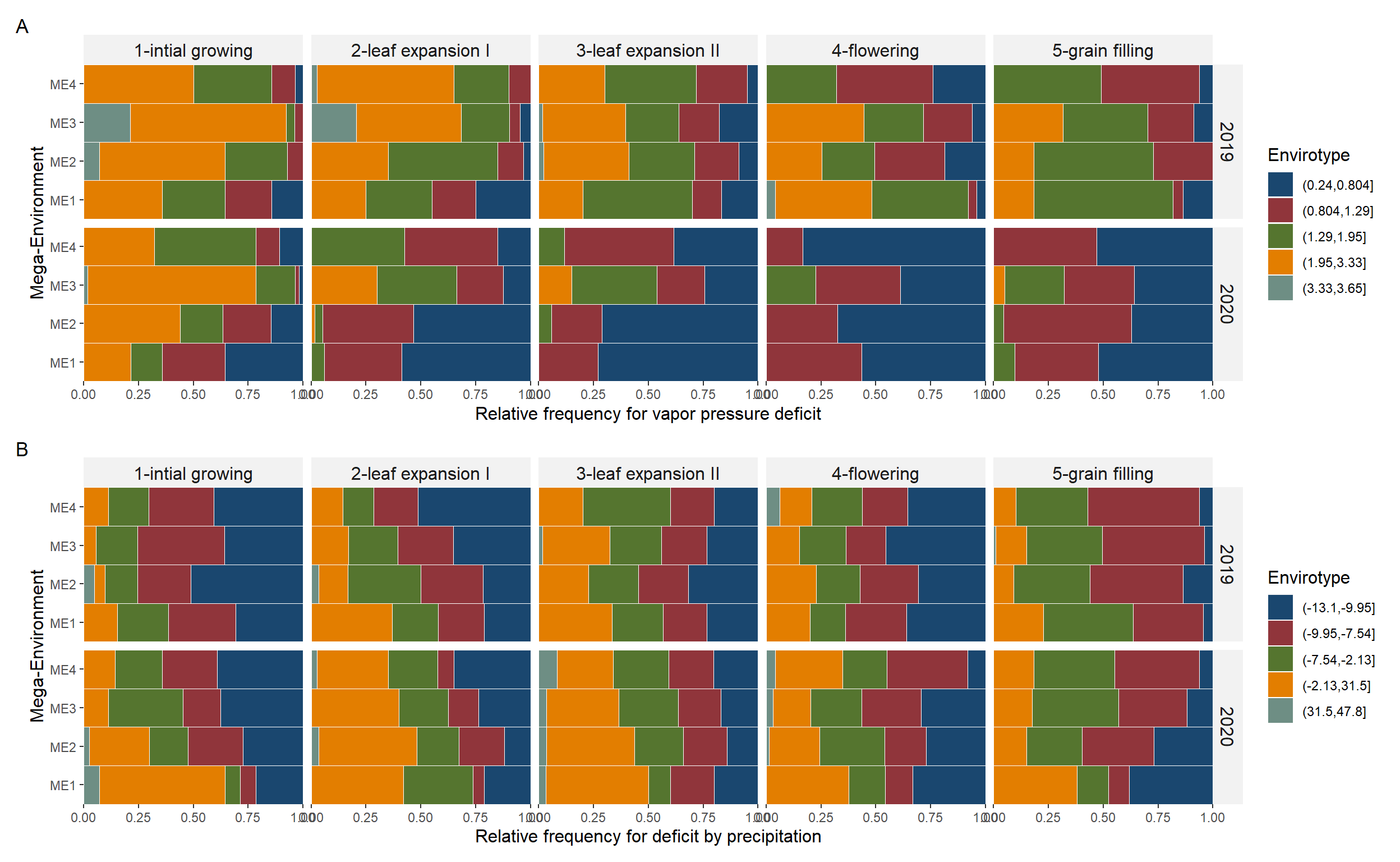
Figure 5.2: Quantiles for vapor pressure deficit (A), deficit by precipitation (B), minimum air temperature (C), and maximum air temperature (D) observed in the studied mega-environments across distinct crop stages and cultivation years.
ggsave("figs/fig4_typology_vpd.jpeg", width = 10, height = 5)6 Helper functions
# get variance components
get_vcomp <- function(model){
  model |>
    tidy(effects = "ran_pars") |>
    mutate(variance = estimate ^ 2) |>
    dplyr::select(group, variance)
}

# get lrt
get_lrt <- function(model){
  model |>
    ranova() |>
    as.data.frame() |>
    mutate(p_val = `Pr(>Chisq)`) |>
    rownames_to_column("term") |>
    dplyr::select(term, AIC, LRT, p_val) |>
    mutate(term = str_sub(term, start = 6, end = -2))
}
7 Models
# fitted models
mod <-
  df_traits_long |>
  group_by(name) |>
  select(-REP) |>
  rename(REP = REP2) |>
  doo(~ lmer(value ~ (1|ME) +   (1|GEN) + (1|GEN:YEAR) + (1|GEN:ME) + (1|GEN:ME:YEAR) + (1|YEAR/ME/REP),
             data = .))
7.0.1 lrt
lrt <-
  mod |>
  mutate(ranova = map(data, ~.x |> get_lrt())) |>
  dplyr::select(-data) |>
  unnest(ranova)

lrt_wide <-
  lrt |>
  dplyr::select(name, term, p_val) |>
  remove_rows_na() |>
  pivot_wider(names_from = name, values_from = p_val)

export(lrt_wide, "data/lrt.xlsx")
7.1 variance component
# vcomp
vcomp <-
  mod |>
  mutate(vcomp = map(data, ~.x |> get_vcomp())) |>
  dplyr::select(-data) |>
  unnest(vcomp) |>
  mutate(group = fct_relevel(group, "YEAR", "ME", "ME:YEAR", "GEN", "GEN:YEAR", "GEN:ME", "GEN:ME:YEAR", "REP:(ME:YEAR)", "Residual"))

vcomp_wide <-
  vcomp |>
  pivot_wider(names_from = name, values_from = variance)

export(vcomp_wide, "data/vcomp_wide.xlsx")

p1 <-
  ggplot(vcomp, aes(name, variance, fill = group)) +
  geom_bar(stat = "identity",
           position = "fill",
           color = "white",
           width = 1) +
  my_theme +
  theme(legend.position = "right") +
  scale_x_discrete(expand = expansion(0)) +
  scale_y_continuous(expand = expansion(0),
                     labels = scales::label_percent()) +
  ggthemes::scale_fill_stata() +
  labs(x = "Traits",
       y = "Percentage of the variance of phenotypic mean values (%)",
       fill = "Source")


vcomp_mean <-
  import("data/h_mean.xlsx") |>
  pivot_longer(-group)

p2 <-
  ggplot(vcomp_mean, aes(name, value, fill = group)) +
  geom_bar(stat = "identity",
           position = "fill",
           color = "white",
           width = 1) +
  my_theme +
  theme(legend.position = "right") +
  scale_x_discrete(expand = expansion(0)) +
  scale_y_continuous(expand = expansion(0),
                     labels = scales::label_percent()) +
  ggthemes::scale_fill_stata() +
  labs(x = "Traits",
       y = "Percentage of the variance of a genotype mean (%)",
       fill = "Source")


arrange_ggplot(p1, p2,
               tag_levels = "A")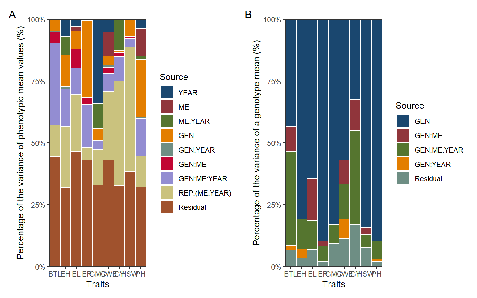
ggsave("figs/fig5_vcomp.jpeg", width = 10, height = 4)8 Selecion within ME
8.1 Stability and mean performance
waas <-
  df_traits_long |>
  dplyr::select(-REP) |>
  pivot_wider(names_from = name, values_from = value) |>
  group_by(ME) |>
  doo(~mps(.,
           env = YEAR,
           gen = GEN,
           rep = REP2,
           resp = GMC:HSW,
           ideotype_mper = c("l, l, l, l, h, h, h, h, h"),
           wmper = 70,
           performance = "blueg",
           stability = "ecovalence"))
## Evaluating trait GMC |=====                                      | 11% 00:00:00
Evaluating trait PH |==========                                  | 22% 00:00:01
Evaluating trait EH |===============                             | 33% 00:00:02
Evaluating trait BTL |===================                        | 44% 00:00:02
Evaluating trait GY |========================                    | 56% 00:00:03
Evaluating trait EL |=============================               | 67% 00:00:04
Evaluating trait ER |==================================          | 78% 00:00:05
Evaluating trait GWE |======================================     | 89% 00:00:05
Evaluating trait HSW |===========================================| 100% 00:00:06
## ---------------------------------------------------------------------------
## P-values for Likelihood Ratio Test of the analyzed traits
## ---------------------------------------------------------------------------
##     model      GMC      PH     EH      BTL       GY       EL       ER      GWE
##  COMPLETE       NA      NA     NA       NA       NA       NA       NA       NA
##       GEN 1.00e+00 0.10506 0.1631 3.95e-01 8.78e-01 1.00e+00 0.498397 7.43e-01
##   GEN:ENV 7.94e-13 0.00307 0.0303 5.16e-09 1.83e-11 2.62e-09 0.000455 2.09e-06
##       HSW
##        NA
##  0.039493
##  0.000391
## ---------------------------------------------------------------------------
## All variables with significant (p < 0.05) genotype-vs-environment interaction
## Evaluating trait GMC |=====                                      | 11% 00:00:00
Evaluating trait PH |==========                                  | 22% 00:00:01
Evaluating trait EH |===============                             | 33% 00:00:02
Evaluating trait BTL |===================                        | 44% 00:00:03
Evaluating trait GY |========================                    | 56% 00:00:04
Evaluating trait EL |=============================               | 67% 00:00:04
Evaluating trait ER |==================================          | 78% 00:00:05
Evaluating trait GWE |======================================     | 89% 00:00:06
Evaluating trait HSW |===========================================| 100% 00:00:07
## ---------------------------------------------------------------------------
## P-values for Likelihood Ratio Test of the analyzed traits
## ---------------------------------------------------------------------------
##     model      GMC       PH       EH      BTL       GY       EL       ER
##  COMPLETE       NA       NA       NA       NA       NA       NA       NA
##       GEN 0.000199 3.23e-04 1.14e-08 3.13e-03 1.00e+00 1.04e-03 1.86e-07
##   GEN:ENV 0.498566 9.27e-12 5.89e-01 5.82e-08 4.17e-19 2.77e-06 1.28e-08
##      GWE      HSW
##       NA       NA
##  0.10611 0.000219
##  0.00134 0.005713
## ---------------------------------------------------------------------------
## Variables with nonsignificant GxE interaction
## GMC EH
## ---------------------------------------------------------------------------
## Evaluating trait GMC |=====                                      | 11% 00:00:00
Evaluating trait PH |==========                                  | 22% 00:00:01
Evaluating trait EH |===============                             | 33% 00:00:02
Evaluating trait BTL |===================                        | 44% 00:00:03
Evaluating trait GY |========================                    | 56% 00:00:04
Evaluating trait EL |=============================               | 67% 00:00:05
Evaluating trait ER |==================================          | 78% 00:00:06
Evaluating trait GWE |======================================     | 89% 00:00:07
Evaluating trait HSW |===========================================| 100% 00:00:07
## ---------------------------------------------------------------------------
## P-values for Likelihood Ratio Test of the analyzed traits
## ---------------------------------------------------------------------------
##     model    GMC       PH       EH      BTL     GY       EL       ER     GWE
##  COMPLETE     NA       NA       NA       NA     NA       NA       NA      NA
##       GEN 0.0192 1.42e-01 1.00e+00 3.93e-01 0.0304 1.21e-05 2.46e-03 0.00268
##   GEN:ENV 0.0272 5.00e-39 3.41e-54 2.63e-13 0.6837 1.00e+00 1.16e-10 0.18759
##    HSW
##     NA
##  0.207
##  0.275
## ---------------------------------------------------------------------------
## Variables with nonsignificant GxE interaction
## GY EL GWE HSW
## ---------------------------------------------------------------------------
## Evaluating trait GMC |=====                                      | 11% 00:00:00
Evaluating trait PH |==========                                  | 22% 00:00:01
Evaluating trait EH |===============                             | 33% 00:00:02
Evaluating trait BTL |===================                        | 44% 00:00:03
Evaluating trait GY |========================                    | 56% 00:00:03
Evaluating trait EL |=============================               | 67% 00:00:04
Evaluating trait ER |==================================          | 78% 00:00:05
Evaluating trait GWE |======================================     | 89% 00:00:05
Evaluating trait HSW |===========================================| 100% 00:00:06
## ---------------------------------------------------------------------------
## P-values for Likelihood Ratio Test of the analyzed traits
## ---------------------------------------------------------------------------
##     model      GMC       PH       EH      BTL       GY       EL        ER
##  COMPLETE       NA       NA       NA       NA       NA       NA        NA
##       GEN 3.03e-01 3.22e-06 6.33e-03 8.33e-01 9.93e-02 4.52e-02  6.33e-04
##   GEN:ENV 2.74e-90 1.07e-52 6.55e-94 4.27e-44 2.07e-82 8.92e-64 1.37e-125
##        GWE      HSW
##         NA       NA
##   8.41e-01 5.12e-03
##  1.81e-115 1.14e-57
## ---------------------------------------------------------------------------
## All variables with significant (p < 0.05) genotype-vs-environment interaction
8.2 Scenarios varying the weight for mean performance and stability
scenarios <-
  waas %>%
  mutate(scenarios = map(data, ~.x %>% wsmp))

saveRDS(scenarios, "data/scenarios.RData")
8.3 Join the WAASBY for all traits
# mean performance and stability
mper <-
  waas %>%
  mutate(mps = map(data, ~.x %>% .[["mps_ind"]])) |>
  unnest(mps) |>
  dplyr::select(-data) |>
  nest(data = GEN:HSW)

## MGIDI applied to the WAASBY values (all)
mgidi <-
  mper |>
  mutate(mgidi = map(data,
                     ~.x |>
                       column_to_rownames("GEN") |>
                       mgidi(SI = 25,
                             weights = c(1,1,1,1,5,1,1,1,1))))
##
## -------------------------------------------------------------------------------
## Principal Component Analysis
## -------------------------------------------------------------------------------
## # A tibble: 9 × 4
##   PC    Eigenvalues `Variance (%)` `Cum. variance (%)`
##   <chr>       <dbl>          <dbl>               <dbl>
## 1 PC1          2.9           32.3                 32.3
## 2 PC2          1.66          18.4                 50.7
## 3 PC3          1.25          13.9                 64.6
## 4 PC4          1.03          11.4                 76.1
## 5 PC5          0.84           9.32                85.4
## 6 PC6          0.51           5.71                91.1
## 7 PC7          0.44           4.85                96.0
## 8 PC8          0.24           2.61                98.6
## 9 PC9          0.13           1.43               100
## -------------------------------------------------------------------------------
## Factor Analysis - factorial loadings after rotation-
## -------------------------------------------------------------------------------
## # A tibble: 9 × 7
##   VAR     FA1   FA2   FA3   FA4 Communality Uniquenesses
##   <chr> <dbl> <dbl> <dbl> <dbl>       <dbl>        <dbl>
## 1 GMC   -0.04  0.06 -0.82  0.15        0.7          0.3
## 2 PH    -0.74 -0.13  0.44 -0.3         0.84         0.16
## 3 EH    -0.88  0    -0.09 -0.08        0.78         0.22
## 4 BTL   -0.34  0.23  0.79  0.09        0.8          0.2
## 5 GY    -0.21 -0.89 -0.03  0.07        0.84         0.16
## 6 EL     0.36 -0.54 -0.16  0.49        0.69         0.31
## 7 ER    -0.16  0.53 -0.55  0.23        0.66         0.34
## 8 GWE    0.04 -0.18  0.01  0.92        0.88         0.12
## 9 HSW    0.36  0.24 -0.24  0.63        0.65         0.35
## -------------------------------------------------------------------------------
## Comunalit Mean: 0.7607318
## -------------------------------------------------------------------------------
## Selection differential
## -------------------------------------------------------------------------------
## # A tibble: 9 × 8
##   VAR   Factor    Xo    Xs    SD SDperc sense     goal
##   <chr> <chr>  <dbl> <dbl> <dbl>  <dbl> <chr>    <dbl>
## 1 PH    FA1     65.9  70.1  4.21   6.39 increase   100
## 2 EH    FA1     64.0  69.4  5.42   8.46 increase   100
## 3 GY    FA2     75.0  86.9 11.9   15.9  increase   100
## 4 EL    FA2     66.4  83.1 16.8   25.3  increase   100
## 5 GMC   FA3     55.1  63.2  8.08  14.7  increase   100
## 6 BTL   FA3     65.1  57.8 -7.33 -11.3  increase     0
## 7 ER    FA3     59.5  56.8 -2.80  -4.70 increase     0
## 8 GWE   FA4     50.0  58.2  8.18  16.3  increase   100
## 9 HSW   FA4     67.9  71.2  3.29   4.85 increase   100
## ------------------------------------------------------------------------------
## Selected genotypes
## -------------------------------------------------------------------------------
## G10 G23 G22 G6 G25 G5
## -------------------------------------------------------------------------------
##
## -------------------------------------------------------------------------------
## Principal Component Analysis
## -------------------------------------------------------------------------------
## # A tibble: 9 × 4
##   PC    Eigenvalues `Variance (%)` `Cum. variance (%)`
##   <chr>       <dbl>          <dbl>               <dbl>
## 1 PC1          2.63          29.2                 29.2
## 2 PC2          1.46          16.3                 45.4
## 3 PC3          1.39          15.5                 60.9
## 4 PC4          1.16          12.9                 73.8
## 5 PC5          0.91          10.1                 83.9
## 6 PC6          0.7            7.73                91.6
## 7 PC7          0.44           4.88                96.5
## 8 PC8          0.23           2.55                99.1
## 9 PC9          0.08           0.94               100
## -------------------------------------------------------------------------------
## Factor Analysis - factorial loadings after rotation-
## -------------------------------------------------------------------------------
## # A tibble: 9 × 7
##   VAR     FA1   FA2   FA3   FA4 Communality Uniquenesses
##   <chr> <dbl> <dbl> <dbl> <dbl>       <dbl>        <dbl>
## 1 GMC    0.65  0.35 -0.5   0.11        0.81         0.19
## 2 PH     0.74 -0.5   0.28  0.13        0.88         0.12
## 3 EH     0.92 -0.14  0.1  -0.05        0.88         0.12
## 4 BTL   -0.1   0.45  0.55 -0.04        0.51         0.49
## 5 GY     0     0.81  0.06 -0.03        0.66         0.34
## 6 EL    -0.21  0.21 -0.16 -0.86        0.86         0.14
## 7 ER    -0.2   0.06 -0.87 -0.07        0.81         0.19
## 8 GWE   -0.29  0.42 -0.2   0.67        0.75         0.25
## 9 HSW   -0.15  0.67 -0.02  0.03        0.47         0.53
## -------------------------------------------------------------------------------
## Comunalit Mean: 0.7376805
## -------------------------------------------------------------------------------
## Selection differential
## -------------------------------------------------------------------------------
## # A tibble: 9 × 8
##   VAR   Factor    Xo    Xs     SD SDperc sense     goal
##   <chr> <chr>  <dbl> <dbl>  <dbl>  <dbl> <chr>    <dbl>
## 1 GMC   FA1     62.5  76.9  14.4   23.1  increase   100
## 2 PH    FA1     61.5  47.5 -14.0  -22.8  increase     0
## 3 EH    FA1     53.0  52.0  -1.01  -1.91 increase     0
## 4 GY    FA2     62.5  88.3  25.8   41.3  increase   100
## 5 HSW   FA2     65.2  90.6  25.4   39.0  increase   100
## 6 BTL   FA3     73.6  80.9   7.32   9.94 increase   100
## 7 ER    FA3     55.9  63.6   7.72  13.8  increase   100
## 8 EL    FA4     56.9  61.3   4.43   7.78 increase   100
## 9 GWE   FA4     57.2  66.6   9.31  16.3  increase   100
## ------------------------------------------------------------------------------
## Selected genotypes
## -------------------------------------------------------------------------------
## G25 G4 G23 G2 G21 G24
## -------------------------------------------------------------------------------
##
## -------------------------------------------------------------------------------
## Principal Component Analysis
## -------------------------------------------------------------------------------
## # A tibble: 9 × 4
##   PC    Eigenvalues `Variance (%)` `Cum. variance (%)`
##   <chr>       <dbl>          <dbl>               <dbl>
## 1 PC1          2.67          29.7                 29.7
## 2 PC2          1.96          21.8                 51.5
## 3 PC3          1.31          14.6                 66.1
## 4 PC4          1.08          12.0                 78.1
## 5 PC5          0.68           7.53                85.6
## 6 PC6          0.52           5.79                91.4
## 7 PC7          0.45           5.01                96.4
## 8 PC8          0.2            2.17                98.6
## 9 PC9          0.13           1.41               100
## -------------------------------------------------------------------------------
## Factor Analysis - factorial loadings after rotation-
## -------------------------------------------------------------------------------
## # A tibble: 9 × 7
##   VAR     FA1   FA2   FA3   FA4 Communality Uniquenesses
##   <chr> <dbl> <dbl> <dbl> <dbl>       <dbl>        <dbl>
## 1 GMC   -0.83  0.23  0.01 -0.16        0.77         0.23
## 2 PH    -0.73 -0.2  -0.07  0.22        0.62         0.38
## 3 EH    -0.76  0.16  0.02  0.44        0.8          0.2
## 4 BTL    0.06 -0.88  0.03 -0.03        0.78         0.22
## 5 GY    -0.01  0.13  0.06 -0.91        0.85         0.15
## 6 EL    -0.04 -0.18 -0.92  0.03        0.88         0.12
## 7 ER     0.08  0.81  0.27 -0.35        0.86         0.14
## 8 GWE    0.3   0.12 -0.57 -0.62        0.82         0.18
## 9 HSW    0.64  0.32 -0.33  0.18        0.65         0.35
## -------------------------------------------------------------------------------
## Comunalit Mean: 0.7809373
## -------------------------------------------------------------------------------
## Selection differential
## -------------------------------------------------------------------------------
## # A tibble: 9 × 8
##   VAR   Factor    Xo    Xs      SD  SDperc sense     goal
##   <chr> <chr>  <dbl> <dbl>   <dbl>   <dbl> <chr>    <dbl>
## 1 GMC   FA1     51.6  68.5  16.9    32.7   increase   100
## 2 PH    FA1     62.5  68.1   5.60    8.96  increase   100
## 3 EH    FA1     51.4  51.8   0.388   0.755 increase   100
## 4 HSW   FA1     73.8  59.9 -14.0   -18.9   increase     0
## 5 BTL   FA2     79.2  85.1   5.90    7.45  increase   100
## 6 ER    FA2     61.2  60.5  -0.764  -1.25  increase     0
## 7 EL    FA3     59.3  60.8   1.49    2.52  increase   100
## 8 GY    FA4     67.4  83.3  16.0    23.7   increase   100
## 9 GWE   FA4     61.0  71.3  10.3    16.9   increase   100
## ------------------------------------------------------------------------------
## Selected genotypes
## -------------------------------------------------------------------------------
## G5 G11 G6 G4 G15 G9
## -------------------------------------------------------------------------------
##
## -------------------------------------------------------------------------------
## Principal Component Analysis
## -------------------------------------------------------------------------------
## # A tibble: 9 × 4
##   PC    Eigenvalues `Variance (%)` `Cum. variance (%)`
##   <chr>       <dbl>          <dbl>               <dbl>
## 1 PC1          2.29          25.5                 25.5
## 2 PC2          1.88          20.9                 46.4
## 3 PC3          1.38          15.4                 61.7
## 4 PC4          1.07          11.9                 73.6
## 5 PC5          0.73           8.06                81.7
## 6 PC6          0.63           7                   88.7
## 7 PC7          0.51           5.61                94.3
## 8 PC8          0.32           3.59                97.9
## 9 PC9          0.19           2.09               100
## -------------------------------------------------------------------------------
## Factor Analysis - factorial loadings after rotation-
## -------------------------------------------------------------------------------
## # A tibble: 9 × 7
##   VAR     FA1   FA2   FA3   FA4 Communality Uniquenesses
##   <chr> <dbl> <dbl> <dbl> <dbl>       <dbl>        <dbl>
## 1 GMC   -0.58 -0.36  0.27 -0.5         0.79         0.21
## 2 PH     0     0.76  0.34 -0.31        0.78         0.22
## 3 EH    -0.03  0.82  0.02  0.12        0.69         0.31
## 4 BTL    0.82 -0.31 -0.01 -0.03        0.77         0.23
## 5 GY     0.8   0.02  0.27 -0.06        0.72         0.28
## 6 EL    -0.08 -0.17  0.1   0.85        0.78         0.22
## 7 ER    -0.1  -0.08 -0.87 -0.1         0.79         0.21
## 8 GWE    0.59  0.05 -0.52  0.07        0.62         0.38
## 9 HSW    0.2  -0.65  0.32  0.36        0.69         0.31
## -------------------------------------------------------------------------------
## Comunalit Mean: 0.7364107
## -------------------------------------------------------------------------------
## Selection differential
## -------------------------------------------------------------------------------
## # A tibble: 9 × 8
##   VAR   Factor    Xo    Xs      SD  SDperc sense     goal
##   <chr> <chr>  <dbl> <dbl>   <dbl>   <dbl> <chr>    <dbl>
## 1 GMC   FA1     57.6  44.2 -13.3   -23.2   increase     0
## 2 BTL   FA1     65.0  93.7  28.7    44.2   increase   100
## 3 GY    FA1     69.1  89.9  20.8    30.1   increase   100
## 4 GWE   FA1     45.6  54.3   8.70   19.1   increase   100
## 5 PH    FA2     59.4  59.2  -0.237  -0.399 increase     0
## 6 EH    FA2     62.0  58.4  -3.60   -5.80  increase     0
## 7 HSW   FA2     58.8  66.9   8.10   13.8   increase   100
## 8 ER    FA3     49.0  36.4 -12.6   -25.8   increase     0
## 9 EL    FA4     65.8  64.6  -1.27   -1.92  increase     0
## ------------------------------------------------------------------------------
## Selected genotypes
## -------------------------------------------------------------------------------
## G15 G25 G21 G26 G18 G23
## -------------------------------------------------------------------------------

p1 <- plot(mgidi$mgidi[[1]], SI = 25, y.lab = "MTMPS index")
p2 <- plot(mgidi$mgidi[[2]], SI = 25, y.lab = "MTMPS index")
p3 <- plot(mgidi$mgidi[[3]], SI = 25, y.lab = "MTMPS index")
p4 <- plot(mgidi$mgidi[[4]], SI = 25, y.lab = "MTMPS index")

arrange_ggplot(p1, p2, p3, p4,
               guides = "collect",
               tag_levels = "A",
               ncol = 4)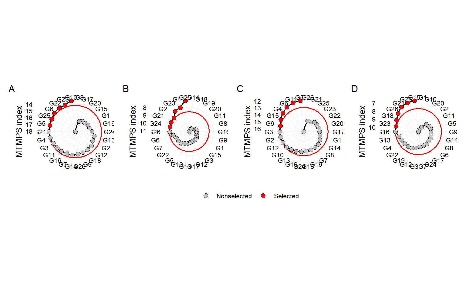
ggsave("figs/fig6_radar.jpeg", width = 12, height = 4)

# selected genotypes
selm1 <- sel_gen(mgidi$mgidi[[1]])
selm2 <- sel_gen(mgidi$mgidi[[2]])
selm3 <- sel_gen(mgidi$mgidi[[3]])
selm4 <- sel_gen(mgidi$mgidi[[4]])


venn_plot(selm1, selm2, selm3, selm4,
          names = c("ME1", "ME2", "ME3", "ME4"),
          show_elements = TRUE) +
  ggthemes::scale_fill_stata()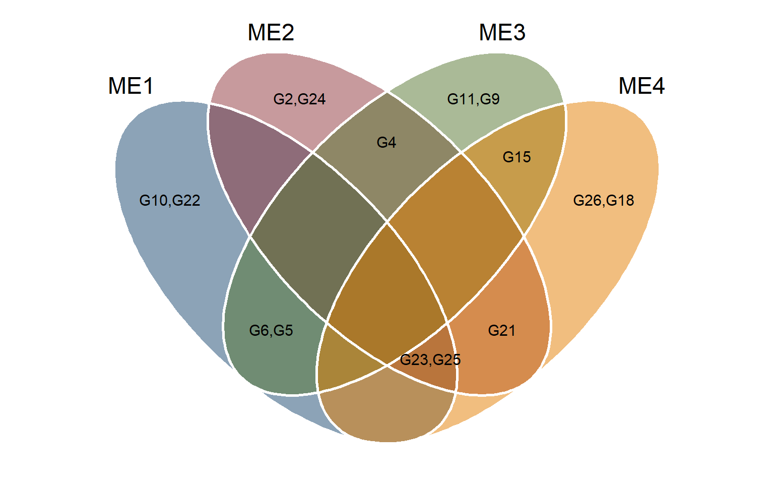
ggsave("figs/fig7_veen.jpeg", width = 6, height = 5)8.4 selection differentials for mean performance
blue_mean <-
  df_traits_long |>
  mean_by(name, ME, GEN, .vars = value)

ovmean <-
  df_traits_long |>
  mean_by(name, ME, .vars = value)

# selected
selected <-
  blue_mean |>
  mutate(selected = case_when(
    ME == "ME1" & GEN %in% selm1 ~ "yes",
    ME == "ME2" & GEN %in% selm2 ~ "yes",
    ME == "ME3" & GEN %in% selm3 ~ "yes",
    ME == "ME4" & GEN %in% selm4 ~ "yes",
    TRUE ~ "no"
  )) |>
  mean_by(name, ME, selected) |>
  filter(selected == "yes")


ds_mper <-
  ovmean |>
  rename(xo = value) |>
  left_join(selected |> rename(xs = value)) |>
  dplyr::select(-selected) |>
  mutate(sd_perc =  (xs - xo) / xo * 100,
         goal = case_when(
           name %in% c("BTL", "EH", "GMC", "PH") ~ "Negative desired gains",
           TRUE ~ "Positive desired gains"
         ),
         negative = ifelse(sd_perc <= 0, "Negative", "Positive"))


ggplot(ds_mper, aes(name, sd_perc)) +
  geom_hline(yintercept = 0, size = 0.2) +
  geom_col(aes(fill = negative),
           col = "black",
           size = 0.2) +
  scale_y_continuous(expand = expansion(mult = 0.2)) +
  facet_nested(~ME + goal, scales = "free_x") +
  geom_text(aes(label = round(sd_perc, 2),
                hjust = ifelse(sd_perc > 0, -0.1, 1.1),
                angle = 90),
            size = 3) +
  labs(x = "Traits",
       y = "Selection differential (%)") +
  my_theme +
  theme(legend.position = "bottom",
        legend.title = element_blank(),
        panel.grid.minor = element_blank()) +
  scale_fill_manual(values = ggthemes::stata_pal()(4)[c(2, 3)])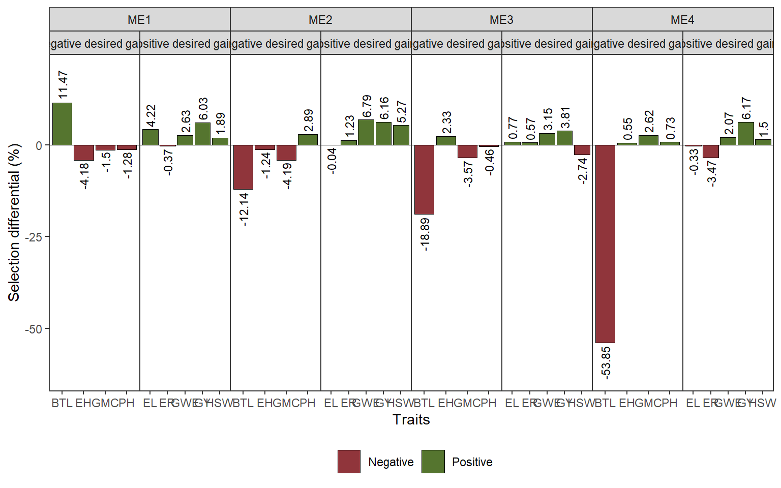
ggsave("figs/fig8_sd_mper.jpeg", width = 14, height = 6)8.5 selection differentials for stability
stab <-
  waas %>%
  mutate(stab = map(data,
                    ~.x %>% .[["stability"]] |>
                      rownames_to_column("GEN"))) |>
  unnest(stab) |>
  dplyr::select(-data) |>
  pivot_longer(GMC:HSW)


stab_ovmean <-
  stab |>
  mean_by(name, ME, .vars = value)

# selected
selected_stab <-
  stab |>
  mutate(selected = case_when(
    ME == "ME1" & GEN %in% selm1 ~ "yes",
    ME == "ME2" & GEN %in% selm2 ~ "yes",
    ME == "ME3" & GEN %in% selm3 ~ "yes",
    ME == "ME4" & GEN %in% selm4 ~ "yes",
    TRUE ~ "no"
  )) |>
  mean_by(name, ME, selected) |>
  filter(selected == "yes")


ds_stab <-
  stab_ovmean |>
  rename(xo = value) |>
  left_join(selected_stab |> rename(xs = value)) |>
  dplyr::select(-selected) |>
  mutate(sd_perc =  (xs - xo) / xo * 100,
         negative = ifelse(sd_perc <= 0, "Negative", "Positive"))

ggplot(ds_stab, aes(name, sd_perc)) +
  geom_hline(yintercept = 0, size = 0.2) +
  geom_col(aes(fill = negative),
           col = "black",
           size = 0.2) +
  scale_y_continuous(expand = expansion(mult = 0.2)) +
  facet_nested(~ME , scales = "free_x") +
  geom_text(aes(label = round(sd_perc, 2),
                hjust = ifelse(sd_perc > 0, -0.1, 1.1),
                angle = 90),
            size = 3) +
  labs(x = "Traits",
       y = "Selection differential (%)") +
  my_theme +
  theme(legend.position = "bottom",
        legend.title = element_blank(),
        panel.grid.minor = element_blank()) +
  scale_fill_manual(values = ggthemes::stata_pal()(4)[c(2, 3)])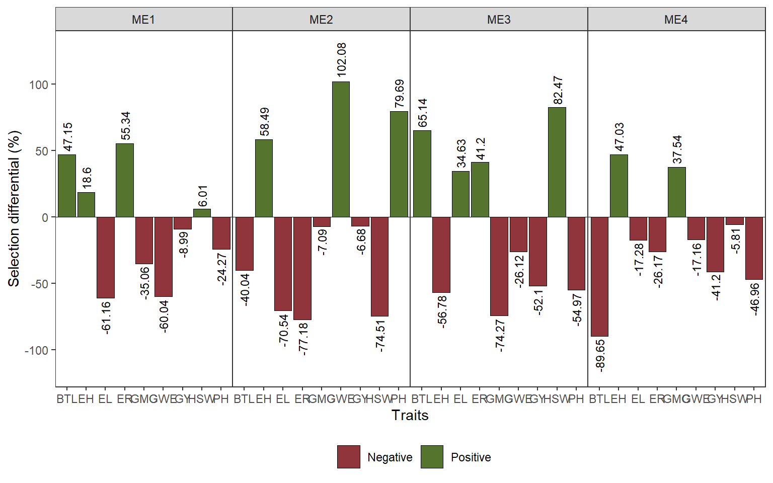
ggsave("figs/fig9_sd_stab.jpeg", width = 14, height = 6)9 Rank winners in each mega-environment
mean_yme <-
  df_traits |>
  mean_by(YEAR, ME, GEN, .vars = GY) |>
  concatenate(ME, YEAR, new_var = ENV)

winners <-
  ge_winners(mean_yme, ME, GEN, GY, type = "ranks") |>
  mutate(id = rep(1:26, 4)) |>
  pivot_wider(names_from = ENV, values_from = GY)
10 GGE
mod_gge <- gge(mean_yme, ME, GEN, GY)

plot(mod_gge, type = 6)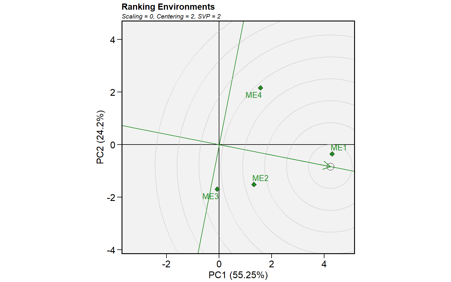
ggsave("figs/fig10_gge.jpeg", width = 10, height = 5)11 Section info
sessionInfo()
## R version 4.2.0 (2022-04-22 ucrt)
## Platform: x86_64-w64-mingw32/x64 (64-bit)
## Running under: Windows 10 x64 (build 22621)
##
## Matrix products: default
##
## locale:
## [1] LC_COLLATE=Portuguese_Brazil.utf8  LC_CTYPE=Portuguese_Brazil.utf8
## [3] LC_MONETARY=Portuguese_Brazil.utf8 LC_NUMERIC=C
## [5] LC_TIME=Portuguese_Brazil.utf8
##
## attached base packages:
## [1] grid      stats     graphics  grDevices utils     datasets  methods
## [8] base
##
## other attached packages:
##  [1] ggsn_0.5.0          forcats_0.5.2       stringr_1.4.1
##  [4] dplyr_1.0.10        purrr_0.3.5         readr_2.1.3
##  [7] tidyr_1.2.1         tibble_3.1.8        tidyverse_1.3.2
## [10] broom.mixed_0.2.9.4 lmerTest_3.1-3      lme4_1.1-31
## [13] Matrix_1.5-3        rnaturalearth_0.1.0 metan_1.17.0.9000
## [16] ggridges_0.5.4      superheat_0.1.0     ggh4x_0.2.3
## [19] ggrepel_0.9.2       FactoMineR_2.6      factoextra_1.0.7
## [22] ggplot2_3.4.0       rio_0.5.29          EnvRtype_1.1.0
##
## loaded via a namespace (and not attached):
##   [1] readxl_1.4.1             backports_1.4.1          systemfonts_1.0.4
##   [4] plyr_1.8.8               sp_1.5-1                 splines_4.2.0
##   [7] listenv_0.8.0            TH.data_1.1-1            digest_0.6.30
##  [10] foreach_1.5.2            htmltools_0.5.3          fansi_1.0.3
##  [13] magrittr_2.0.3           googlesheets4_1.0.1      cluster_2.1.4
##  [16] tzdb_0.3.0               openxlsx_4.2.5.1         globals_0.16.2
##  [19] modelr_0.1.10            sandwich_3.0-2           timechange_0.1.1
##  [22] rmdformats_1.0.4         jpeg_0.1-9               colorspace_2.0-3
##  [25] rvest_1.0.3              textshaping_0.3.6        haven_2.5.1
##  [28] xfun_0.35                crayon_1.5.2             jsonlite_1.8.3
##  [31] iterators_1.0.14         survival_3.3-1           zoo_1.8-11
##  [34] glue_1.6.2               polyclip_1.10-4          gtable_0.3.1
##  [37] gargle_1.2.1             emmeans_1.8.2            car_3.1-1
##  [40] abind_1.4-5              scales_1.2.1             mvtnorm_1.1-3
##  [43] DBI_1.1.3                GGally_2.1.2             rstatix_0.7.1
##  [46] ggthemes_4.2.4           Rcpp_1.0.9               xtable_1.8-4
##  [49] units_0.8-0              flashClust_1.01-2        foreign_0.8-82
##  [52] proxy_0.4-27             DT_0.26                  htmlwidgets_1.5.4
##  [55] httr_1.4.4               RColorBrewer_1.1-3       ellipsis_0.3.2
##  [58] pkgconfig_2.0.3          reshape_0.8.9            farver_2.1.1
##  [61] multcompView_0.1-8       sass_0.4.4               dbplyr_2.2.1
##  [64] utf8_1.2.2               reshape2_1.4.4           labeling_0.4.2
##  [67] tidyselect_1.2.0         rlang_1.0.6              munsell_0.5.0
##  [70] cellranger_1.1.0         tools_4.2.0              cachem_1.0.6
##  [73] cli_3.4.1                generics_0.1.3           ggmap_3.0.1
##  [76] broom_1.0.1              mathjaxr_1.6-0           ggdendro_0.1.23
##  [79] evaluate_0.18            fastmap_1.1.0            ragg_1.2.4
##  [82] yaml_2.3.6               knitr_1.41               fs_1.5.2
##  [85] zip_2.2.2                RgoogleMaps_1.4.5.3      future_1.29.0
##  [88] nlme_3.1-157             leaps_3.1                xml2_1.3.3
##  [91] compiler_4.2.0           rstudioapi_0.14          png_0.1-7
##  [94] curl_4.3.3               ggsignif_0.6.4           e1071_1.7-12
##  [97] reprex_2.0.2             tweenr_2.0.2             bslib_0.4.1
## [100] stringi_1.7.8            highr_0.9                lattice_0.20-45
## [103] rnaturalearthhires_0.2.0 classInt_0.4-8           nloptr_2.0.3
## [106] vctrs_0.5.0              pillar_1.8.1             lifecycle_1.0.3
## [109] furrr_0.3.1              jquerylib_0.1.4          estimability_1.4.1
## [112] maptools_1.1-5           bitops_1.0-7             data.table_1.14.6
## [115] patchwork_1.1.2          R6_2.5.1                 bookdown_0.30
## [118] KernSmooth_2.23-20       parallelly_1.32.1        codetools_0.2-18
## [121] boot_1.3-28              MASS_7.3-58.1            assertthat_0.2.1
## [124] withr_2.5.0              multcomp_1.4-20          parallel_4.2.0
## [127] hms_1.1.2                coda_0.19-4              class_7.3-20
## [130] minqa_1.2.5              rmarkdown_2.18           carData_3.0-5
## [133] googledrive_2.0.0        ggpubr_0.5.0             sf_1.0-9
## [136] ggforce_0.4.1            numDeriv_2016.8-1.1      scatterplot3d_0.3-42
## [139] lubridate_1.9.0