Phytopatometry in R with the package pliman

Getting started

Single images

library(pliman)
#> |==========================================================|
#> | Tools for Plant Image Analysis (pliman 2.1.0)            |
#> | Author: Tiago Olivoto                                    |
#> | Type `citation('pliman')` to know how to cite pliman     |
#> | Visit 'http://bit.ly/pkg_pliman' for a complete tutorial |
#> |==========================================================|
# set the path directory
path_soy <- "https://raw.githubusercontent.com/TiagoOlivoto/images/master/pliman"
# import images
img <- image_import("leaf.jpg", path = path_soy)
healthy <- image_import("healthy.jpg", path = path_soy)
symptoms <- image_import("sympt.jpg", path = path_soy)
background <- image_import("back.jpg", path = path_soy)
image_combine(img, healthy, symptoms, background, ncol = 4)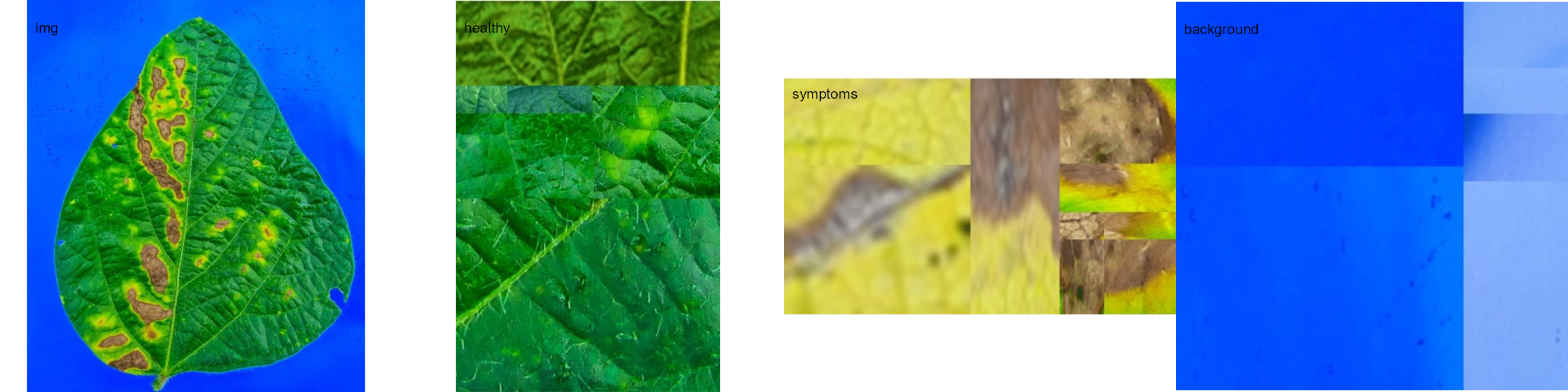

Image palettes

Sample palettes can be created by manually sampling small areas of representative images and producing a composite image that represents each of the desired classes (background, healthy, and symptomatic tissues). Another approach is to use the image_palette() function to generate sample color palettes.

pals <- image_palette(img, npal = 8)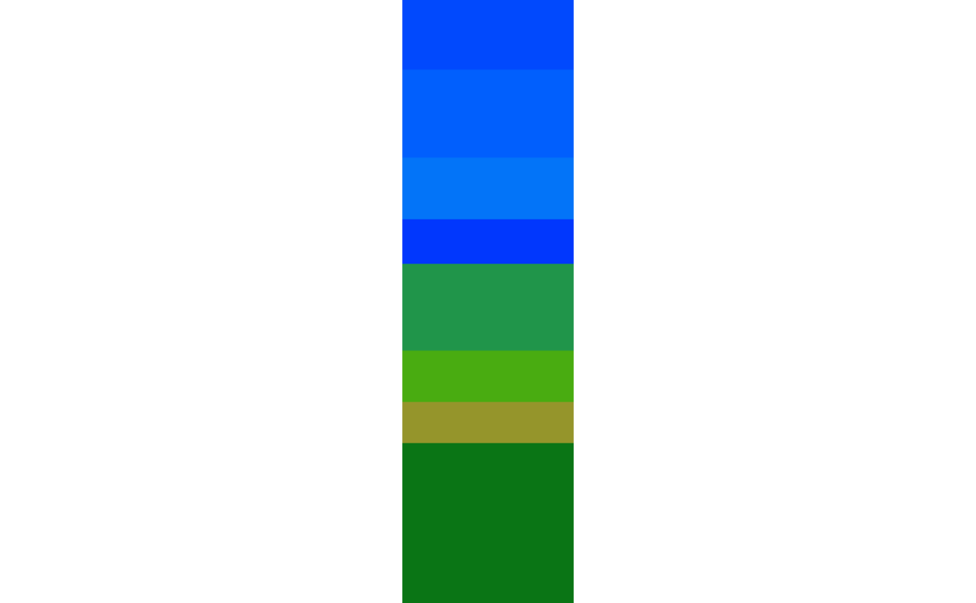

image_combine(pals$palette_list)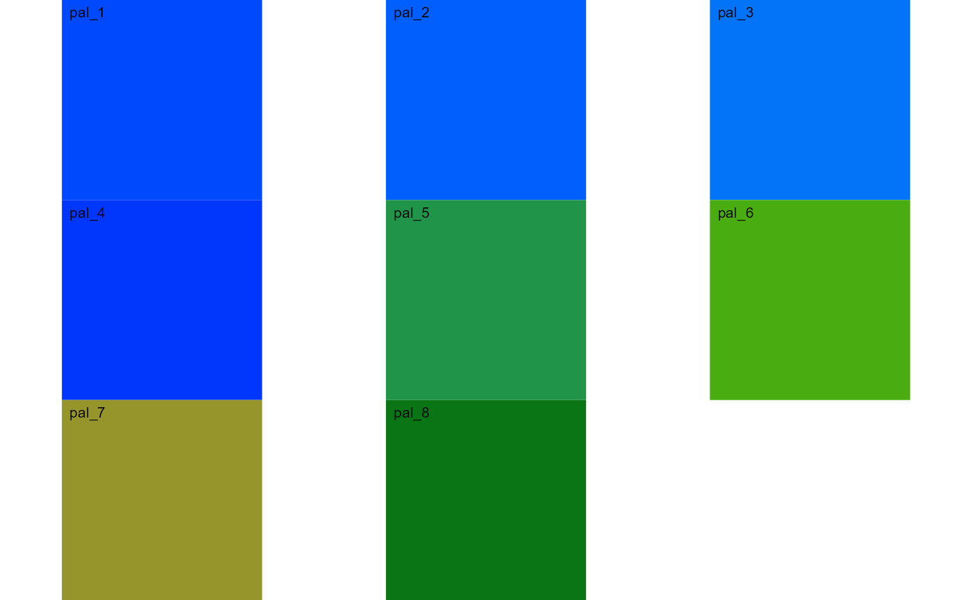

# to extract the color palettes, use the object
plot(pals$palette_list[[1]])

# default settings
res <-
  measure_disease(img = img,
                  img_healthy = healthy,
                  img_symptoms = symptoms,
                  img_background = background)

res$severity
#>    healthy symptomatic
#> 1 89.36756    10.63244

Alternatively, users can create a mask instead of displaying the original image.


# create a personalized mask
res2 <- 
  measure_disease(img = img,
                  img_healthy = healthy,
                  img_symptoms = symptoms,
                  img_background = background,
                  show_original = FALSE, # create a mask
                  show_contour = FALSE, # hide the contour line
                  col_background = "white", # default
                  col_lesions = "red", # default
                  col_leaf = "green") # default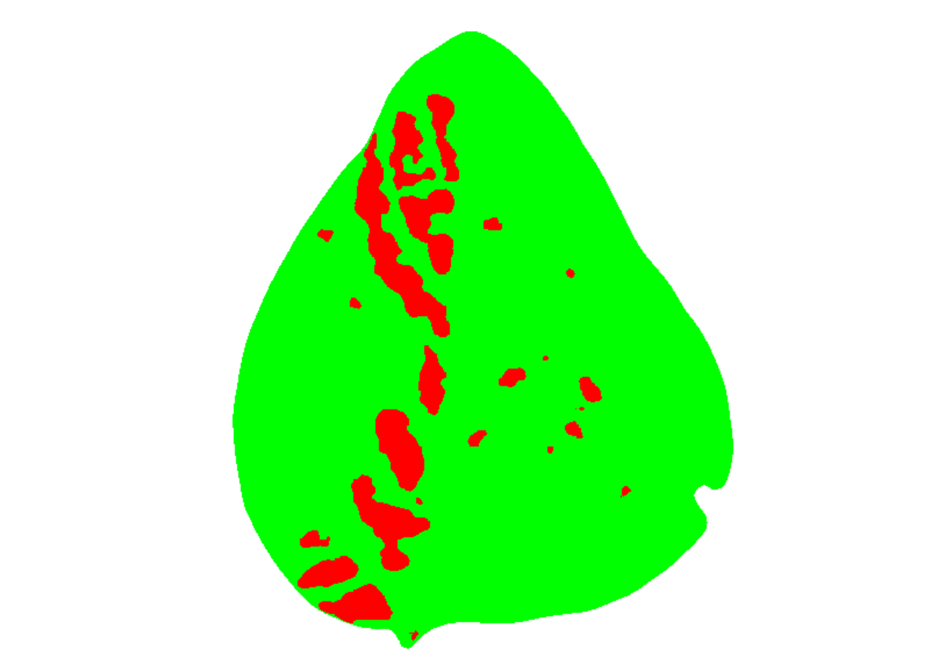



res2$severity
#>    healthy symptomatic
#> 1 89.18203    10.81797

Variations in image palettes

The results may vary depending on how the palettes are chosen and are subjective due to the researcher’s experience. In the following example, I present a second variation in the color palettes, where only the necrotic area is assumed to be the diseased tissue. Therefore, the symptomatic area will be smaller than in the previous example.


# import images
healthy2 <- image_import("healthy2.jpg", path = path_soy)
symptoms2 <- image_import("sympt2.jpg", path = path_soy)
background2 <- image_import("back2.jpg", path = path_soy)
image_combine(healthy2, symptoms2, background2, ncol = 3)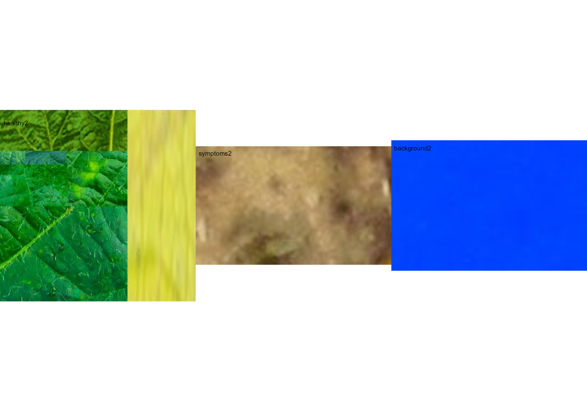


res3 <-
  measure_disease(img = img,
                  img_healthy = healthy2,
                  img_symptoms = symptoms2,
                  img_background = background2)

res3$severity
#>    healthy symptomatic
#> 1 93.62367    6.376329

Lesion features

res4 <-
  measure_disease(img = img,
                  img_healthy = healthy,
                  img_symptoms = symptoms,
                  img_background = background,
                  show_features = TRUE,
                  marker = "area")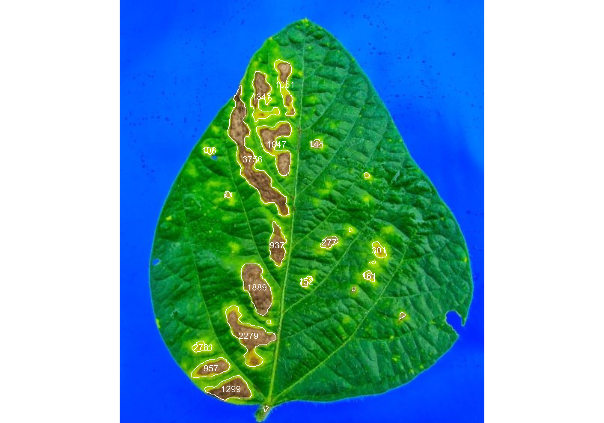

res4$shape
#>    id       mx       my area perimeter radius_mean radius_min radius_max
#> 1   1 221.2854 113.5300 1051 197.61017   22.542426  0.4574999  39.195089
#> 2   2 189.7655 129.4557 1347 255.30866   20.536491  1.9179031  39.047473
#> 3   3 177.9097 213.2194 3756 479.44574   50.429324  1.0172814  94.833036
#> 4   4 209.8348 193.3616 1847 254.82338   24.054797  0.8294188  42.394976
#> 5   5 263.3015 192.5685  144  46.07107    6.432979  4.3560657   8.710006
#> 6   6 119.5133 201.4716  106  37.97056    5.401209  3.2145054   7.011175
#> 8   8 145.0949 260.5257   77  31.72792    4.512716  3.1588917   5.890903
#> 9   9 210.9025 328.1284  937 150.05382   18.551319  7.4968160  30.607324
#> 11 11 280.3690 323.9892  277  66.35534    9.158113  5.3467341  13.132584
#> 12 12 347.0191 334.7505  301  67.52691    9.572126  5.3572461  12.988460
#> 15 15 183.7555 384.4845 1889 195.50967   25.075741 13.1297926  38.817412
#> 16 16 333.3873 369.2890  161  48.45584    6.871599  4.4326658   9.669833
#> 17 17 249.6167 376.2756  152  48.87006    6.729158  3.3320576   9.624262
#> 19 19 172.3420 449.2575 2279 281.59293   28.762923 13.1316755  47.596995
#> 23 23 109.1753 464.1340  278  76.69848    9.163249  3.4697057  13.849439
#> 24 24 122.6784 492.3605  957 134.39697   18.159020  9.9418772  28.187512
#> 25 25 149.1242 520.1696 1299 163.95332   21.132646 11.0804543  32.776744
#>     radius_sd  diam_mean   diam_min  diam_max  maj_axis  min_axis    length
#> 1  11.1940055  45.084852  0.9149997  78.39018 24.256153  6.662562  77.18840
#> 2   9.0513289  41.072981  3.8358061  78.09495 19.657618 10.811397  66.41748
#> 3  25.4996489 100.858648  2.0345627 189.66607 54.980195 12.998467 185.15668
#> 4  10.1985631  48.109595  1.6588377  84.78995 22.418395 13.401467  74.44851
#> 5   1.2327550  12.865958  8.7121315  17.42001  5.395079  3.709751  16.00669
#> 6   1.0981030  10.802418  6.4290108  14.02235  4.348269  3.381714  13.03497
#> 8   0.7570407   9.025432  6.3177834  11.78181  3.602634  2.817621  11.04797
#> 9   6.4909295  37.102638 14.9936320  61.21465 18.026385  7.811137  60.30694
#> 11  2.1249370  18.316226 10.6934682  26.26517  7.999669  4.930767  25.11932
#> 12  2.0917918  19.144253 10.7144923  25.97692  8.298294  5.202436  25.60521
#> 15  7.5163246  50.151482 26.2595852  77.63482 23.128597 12.248413  73.99521
#> 16  1.4614520  13.743197  8.8653316  19.33967  5.796511  3.962867  17.73659
#> 17  1.7310964  13.458317  6.6641152  19.24852  5.976655  3.533626  18.37484
#> 19  9.8848790  57.525846 26.2633511  95.19399 26.433541 15.029328  87.49540
#> 23  2.9122587  18.326497  6.9394113  27.69888  8.354319  4.746453  27.01285
#> 24  5.5924775  36.318041 19.8837544  56.37502 17.082987  8.302549  54.39783
#> 25  6.0669818  42.265293 22.1609087  65.55349 19.277370 10.560426  62.95761
#>        width
#> 1  22.629530
#> 2  37.692131
#> 3  45.978766
#> 4  46.442456
#> 5  10.914290
#> 6   9.824116
#> 8   8.595533
#> 9  23.672188
#> 11 14.846347
#> 12 15.189243
#> 15 34.924170
#> 16 12.080600
#> 17 10.717088
#> 19 54.713490
#> 23 14.982384
#> 24 22.794774
#> 25 32.894039
res4$statistics
#>        stat      value
#> 1         n    17.0000
#> 2  min_area    77.0000
#> 3 mean_area   991.6471
#> 4  max_area  3756.0000
#> 5   sd_area  1009.1980
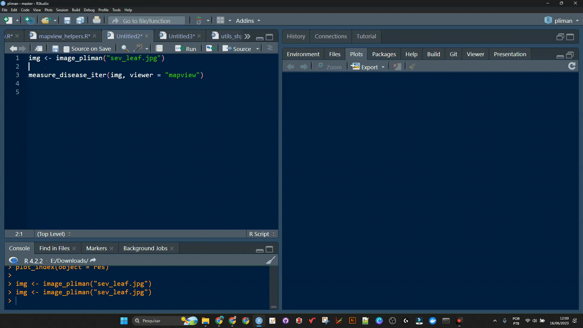
#> 6  sum_area 16858.0000

Interactive disease measurements

An alternative approach to measuring disease percentage is available through the measure_disease_iter() function. This function offers an interactive interface that empowers users to manually select sample colors directly from the image. By doing so, it provides a highly customizable analysis method.

One advantage of using measure_disease_iter() is the ability to utilize the “mapview” viewer, which enhances the analysis process by offering zoom-in options. This feature allows users to closely examine specific areas of the image, enabling detailed inspection and accurate disease measurement.

img <- image_pliman("sev_leaf.jpg", plot = TRUE)
measure_disease_iter(img, viewer = "mapview")

A little bit more!

At this link you will find more examples on how to use {pliman} to analyze plant images. Source code and images can be downloaded here. You can also find a talk (Portuguese language) about {pliman} here. Lights, camera, {pliman}!

Tiago Olivoto

2023-10-22