Getting started
A
polygonis a plane figure that is described by a finite number of straight-line segments connected to form a closed polygonal chain (Singer, 1993)1.
Given the above, we may conclude that image objects can be expressed
as polygons with n vertices. pliman has a set
of useful functions (draw_*()) to draw common shapes such
as circles, squares, triangles, rectangles and n-tagons.
Another group of poly_*() functions can be used to analyze
polygons. Let’s start with a simple example, related to the area and
perimeter of a square.
library(pliman)
#> |==========================================================|
#> | Tools for Plant Image Analysis (pliman 2.1.0)            |
#> | Author: Tiago Olivoto                                    |
#> | Type `citation('pliman')` to know how to cite pliman     |
#> | Visit 'http://bit.ly/pkg_pliman' for a complete tutorial |
#> |==========================================================|
square <- draw_square(side = 1)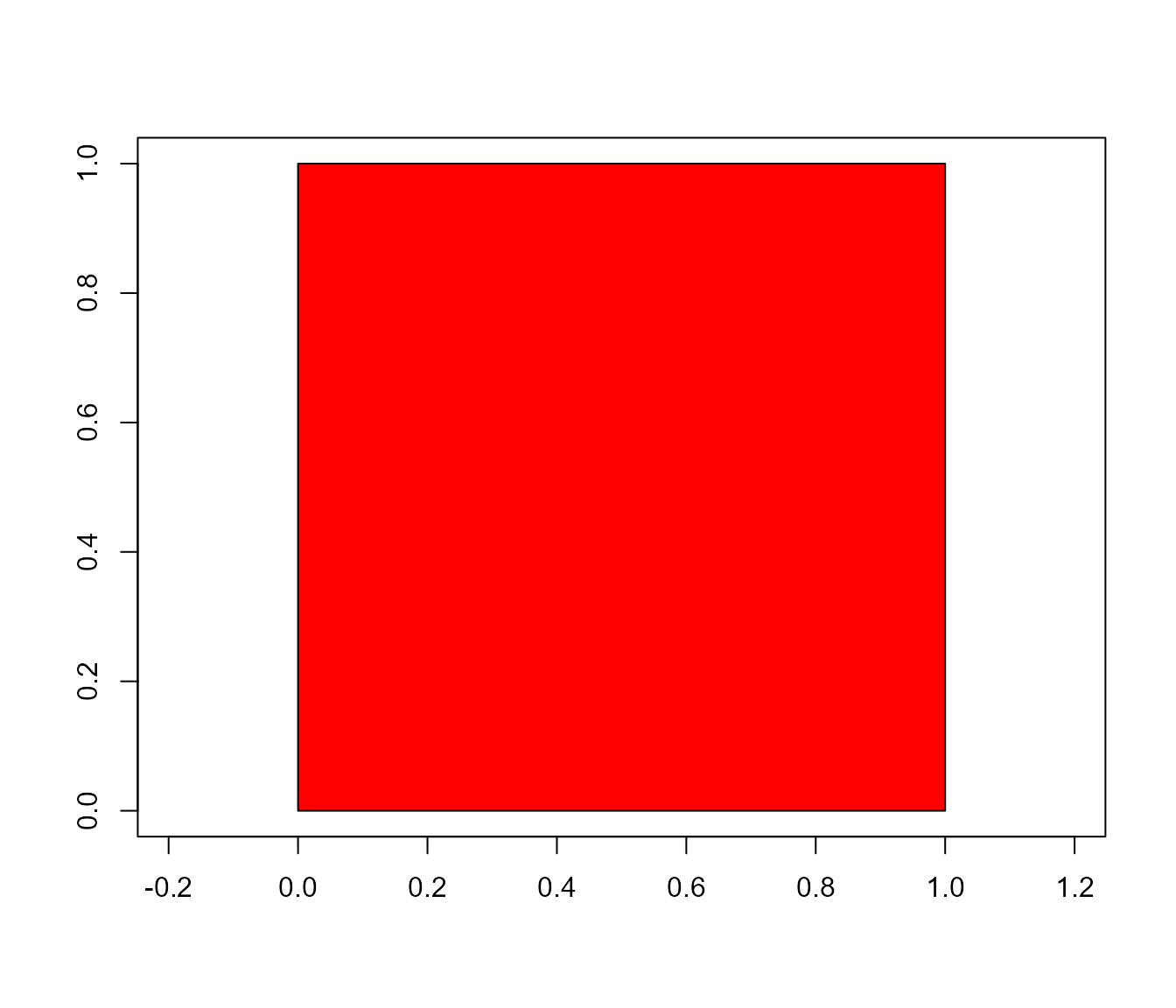
poly_area(square)
#> [1] 1
poly_perimeter(square)
#> [1] 3
Now, Let’s see what happens when we start with a hexagon and increase the number of sides up to 1000.
shapes <- list(side6 <- draw_n_tagon(6, plot = FALSE),
               side12 <- draw_n_tagon(12, plot = FALSE),
               side24 <- draw_n_tagon(24, plot = FALSE),
               side100 <- draw_n_tagon(100, plot = FALSE),
               side500 <- draw_n_tagon(500, plot = FALSE),
               side100 <- draw_n_tagon(1000, plot = FALSE))
plot_polygon(shapes, merge = FALSE)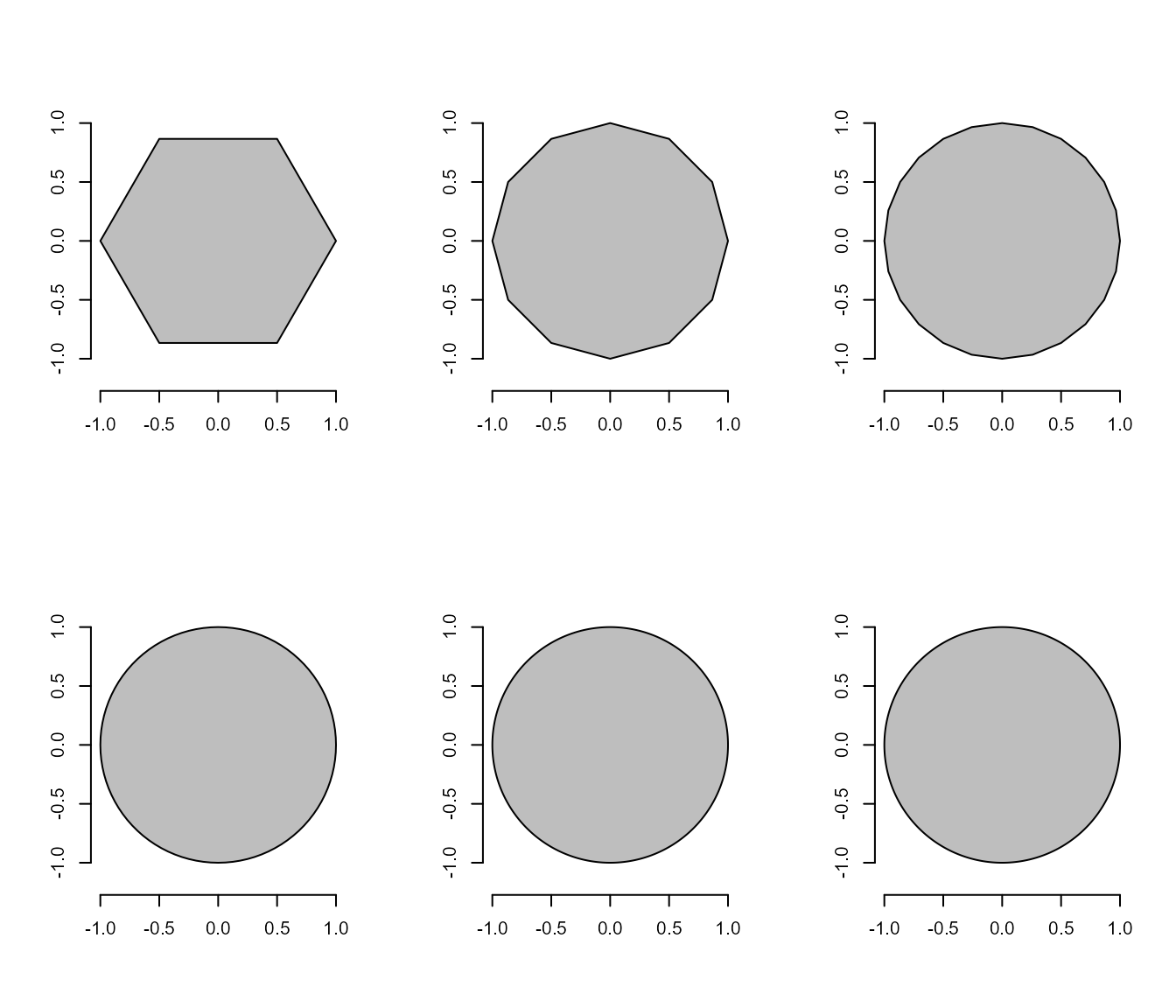
#> [[1]]
#> NULL
#>
#> [[2]]
#> NULL
#>
#> [[3]]
#> NULL
#>
#> [[4]]
#> NULL
#>
#> [[5]]
#> NULL
#>
#> [[6]]
#> NULL

poly_area(shapes)
#> [1] 2.598076 3.000000 3.105829 3.139526 3.141510 3.141572
poly_perimeter(shapes)
#> [1] 5.000000 5.694019 6.004205 6.219330 6.270578 6.276892
Note that when \(n \to \infty\), the
sum of sides becomes the circumference of the circle, given by \(2\pi r\), and the area becomes \(\pi r^2\). This is cool, but
pliman is mainly designed to analyze plant image analysis.
So, why would we use polygons? Let’s see how we can use these functions
to obtain useful information.
link <- "https://raw.githubusercontent.com/TiagoOlivoto/tiagoolivoto/master/static/tutorials/pliman_lca/imgs/leaves.jpg"
leaves <- image_import(link, plot = TRUE)
cont <- object_contour(leaves, watershed = FALSE, index = "HI")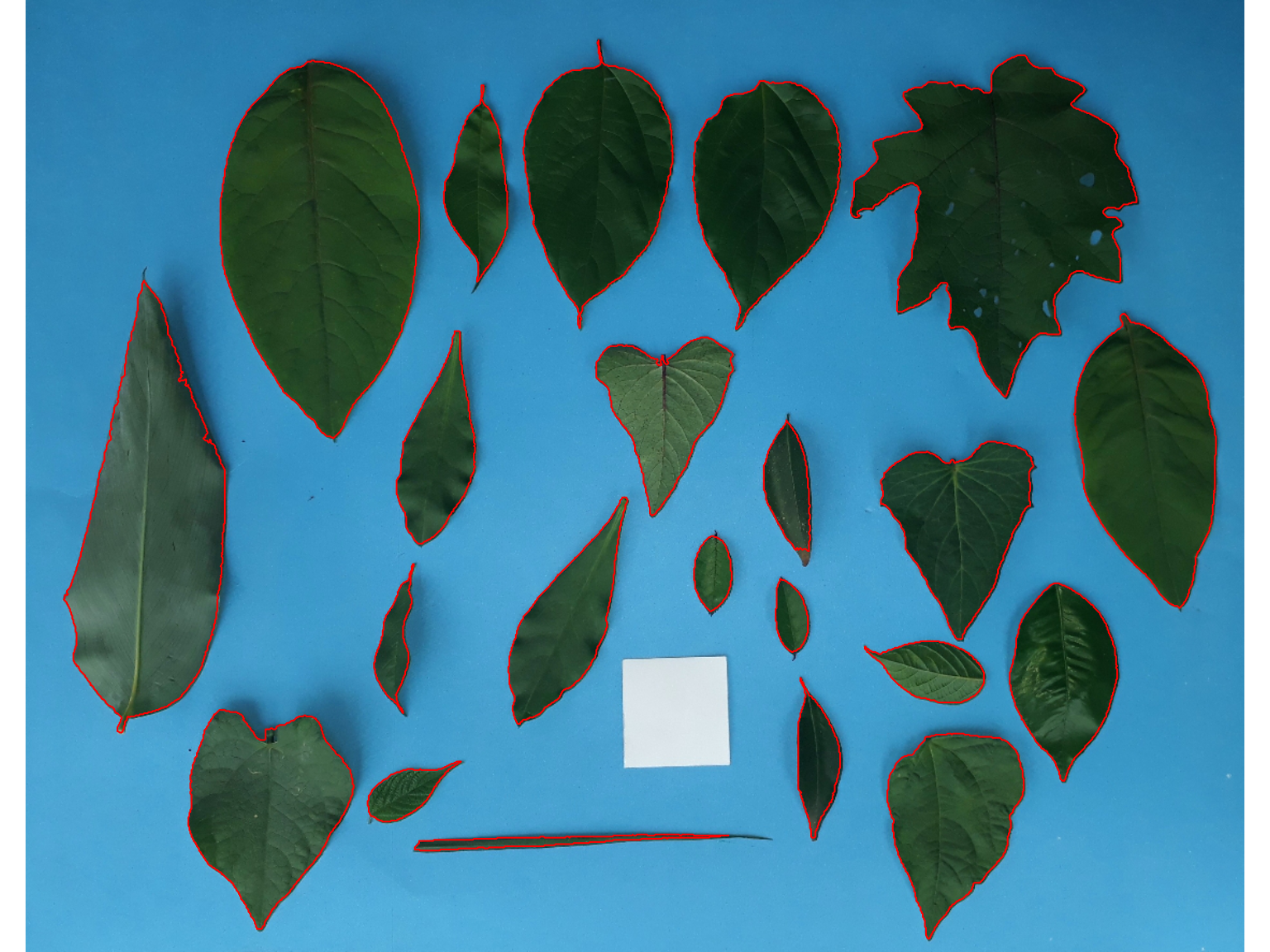
# plotting the polygon
plot_polygon(cont)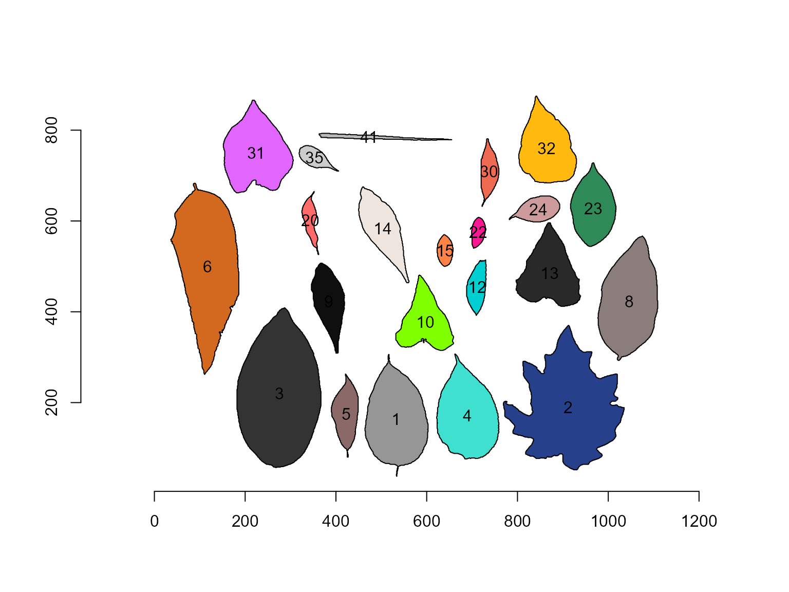
Object measures
Nice! We can use the contour of any object to obtain useful information related to its shape. To reduce the amount of output, I will only use five samples: 2, 4, 13, 24, and 35.
cont <- cont[c("2", "4", "13", "24", "41")]
plot_polygon(cont)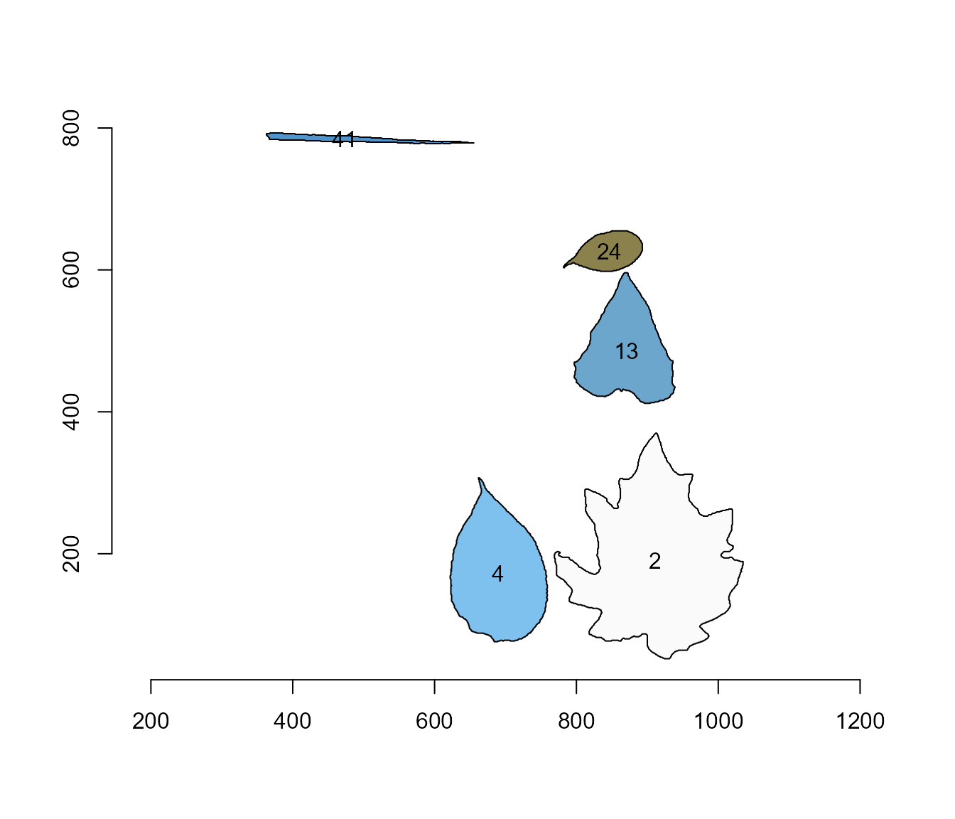
In the current version of pliman, you will be able to
compute the following measures. For more details, see Chen & Wang
(2005)2,
Claude (2008)3, and Montero et al. 20094.
Area
The area of a shape is computed using Shoelace Formula (Lee and Lim, 2017)5, as follows
\[ A=\frac{1}{2}\left|\sum_{i=1}^{n}\left(x_{i} y_{i+1}-x_{i+1}y_{i}\right)\right| \]
poly_area(cont)
#> [1] 45075.0 20793.5 15183.5  4144.0  1688.0
Perimeter
The perimeter is computed as the sum of the euclidean distance
between every point of a shape. The distances can be obtained with
poly_distpts().
poly_perimeter(cont)
#>         2         4        13        24        41
#> 1290.1413  630.7128  565.7422  291.5929  603.1543

# perimeter of a circle with radius equals to 2
circle <- draw_circle(radius = 2, plot = FALSE)
poly_perimeter(circle)
#> [1] 12.56635

# check the result
2*pi*2
#> [1] 12.56637
Radius
The radius of a pixel in the object contour is computed as its
distance to the object centroid (also called as ‘center of mass’). These
distances can be obtained with poly_centdist(). The
average, maximum and minimum radius can be obtained.
dists <- poly_centdist(cont)

# statistics for the radius
mean_list(dists)
#>         2         4        13        24        41
#> 119.55450  85.22870  72.13064  39.10193  73.70601
min_list(dists)
#>         2         4        13        24        41
#> 68.938361 62.146291 48.670983 25.480450  2.638939
max_list(dists)
#>         2         4        13        24        41
#> 171.20105 129.75938 108.46217  61.56336 147.04645
sd_list(dists)
#>        2        4       13       24       41
#> 20.94407 16.84946 14.62283 10.26425 42.27660

# average radius of the circle above
poly_centdist(circle) |> mean_list()
#> [1] 1.999998
Length and width
The length and width of an object are computed with
poly_lw() as the difference between the maximum and minimum
of x and y coordinates after the object has
been aligned with poly_align().
aligned <- poly_align(cont)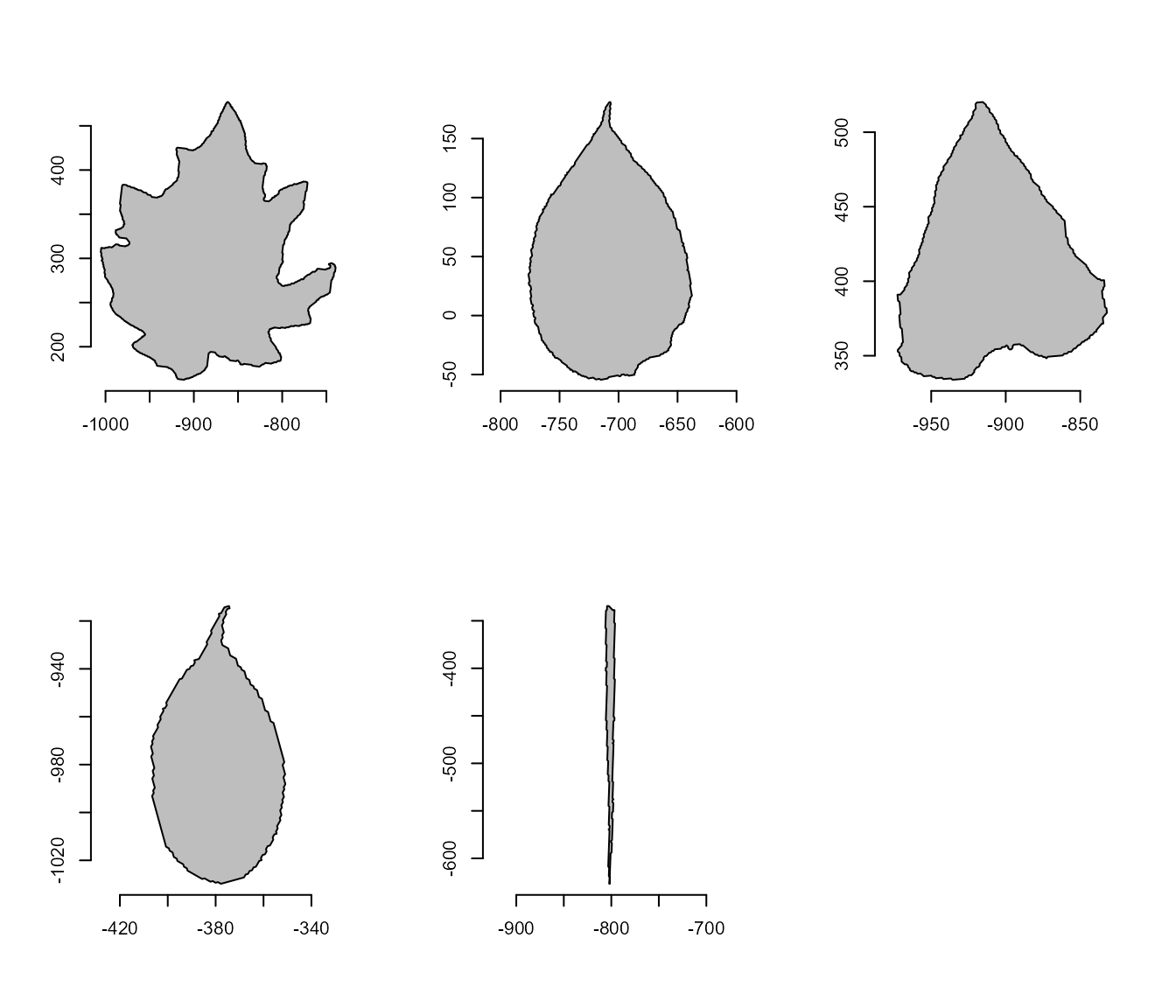
# compute length and width
poly_lw(cont)
#>        length     width
#> [1,] 314.3777 265.87632
#> [2,] 235.4453 138.61494
#> [3,] 186.3901 140.53457
#> [4,] 116.0408  56.15904
#> [5,] 292.2781  10.17229
Circularity, eccentricity, caliper, and elongation
Circularity measure (Montero et al. 2009)6 is also called shape compactness, or roundness measure of an object. It is given by \(C = P^2 / A\), where \(P\) is the perimeter and \(A\) is the area of the object.
poly_circularity(cont)
#>         2         4        13        24        41
#>  36.92656  19.13091  21.07974  20.51796 215.51845
Since the above measure is dependent on the scale, the normalized circularity can be used. In this case, it is assumed to be unity for a circle. This measure is invariant under translation, rotation, scaling transformations, and dimensionless. It is given by: \(Cn = P^2 / 4 \pi A\)
poly_circularity_norm(cont)
#>          2          4         13         24         41
#> 0.34030714 0.65686211 0.59613497 0.61245704 0.05830763

# normalized circularity for different shapes
draw_square(plot = FALSE) |> poly_circularity_norm()
#> [1] 1.396263
draw_circle(plot = FALSE) |> poly_circularity_norm()
#> [1] 0.9999967
poly_circularity_haralick() computes the Haralick’s
circularity (CH). The method is based on the computation of all the
Euclidean distances from the object centroid to each boundary pixel.
With this set of distances, the mean (\(m\)) and the standard deviation (\(s\)) are computed. These statistical
parameters are used on a ratio that calculates the circularity, CH, of a
shape, as \(CH = m/sd\)
poly_circularity_haralick(cont)
#>        2        4       13       24       41
#> 5.708275 5.058245 4.932743 3.809527 1.743423
poly_convexity() Computes the convexity of a shape using
a ratio between the perimeter of the convex hull and the perimeter of
the polygon.
poly_convexity(cont)
#>         2         4        13        24        41
#> 0.6435196 0.8850799 0.7579630 0.9099463 0.7222449
poly_eccentricity() Computes the eccentricity of a shape
using the ratio of the eigenvalues (inertia axes of coordinates).
poly_eccentricity(cont)
#>             [,1]
#> [1,] 0.833397171
#> [2,] 0.421770889
#> [3,] 0.599180391
#> [4,] 0.297943286
#> [5,] 0.001438398
poly_elongation() Computes the elongation of a shape as
1 - width / length
poly_elongation(cont)
#>           [,1]
#> [1,] 0.1542773
#> [2,] 0.4112648
#> [3,] 0.2460192
#> [4,] 0.5160407
#> [5,] 0.9651965
poly_caliper() Computes the caliper (Also called the
Feret’s diameter).
poly_caliper(cont)
#>        2        4       13       24       41
#> 317.5106 229.5125 187.4807 115.1347 253.3338
Users can use the function poly_measures() to compute
most of the object measures in a single call.
(measures <- poly_measures(cont))
#>    id        x        y    area area_ch perimeter radius_mean radius_min
#> 2   1 911.0558 190.1729 45075.0   57540 1290.1413   119.55450  68.938361
#> 4   2 689.1227 171.8705 20793.5   21924  630.7128    85.22870  62.146291
#> 13  3 870.4033 485.5803 15183.5   16554  565.7422    72.13064  48.670983
#> 24  4 846.2110 625.7005  4144.0    4433  291.5929    39.10193  25.480450
#> 41  5 472.9797 784.6601  1688.0    2167  603.1543    73.70601   2.638939
#>    radius_max radius_sd radius_ratio diam_mean   diam_min diam_max  caliper
#> 2   171.20105  20.94407     2.483393 239.10899 137.876721 342.4021 314.3777
#> 4   129.75938  16.84946     2.087967 170.45741 124.292582 259.5188 235.4453
#> 13  108.46217  14.62283     2.228477 144.26129  97.341966 216.9243 186.3901
#> 24   61.56336  10.26425     2.416102  78.20386  50.960900 123.1267 116.0408
#> 41  147.04645  42.27660    55.721805 147.41202   5.277878 294.0929 292.2781
#>      length     width  solidity convexity elongation circularity
#> 2  314.3777 265.87632 0.7833681 0.6435196  0.1542773    36.92656
#> 4  235.4453 138.61494 0.9484355 0.8850799  0.4112648    19.13091
#> 13 186.3901 140.53457 0.9172103 0.7579630  0.2460192    21.07974
#> 24 116.0408  56.15904 0.9348071 0.9099463  0.5160407    20.51796
#> 41 292.2781  10.17229 0.7789571 0.7222449  0.9651965   215.51845
#>    circularity_haralick circularity_norm eccentricity       pcv
#> 2              5.708275       0.34030714  0.833397171 2.6693543
#> 4              5.058245       0.65686211  0.421770889 0.8422071
#> 13             4.932743       0.59613497  0.599180391 1.1910148
#> 24             3.809527       0.61245704  0.297943286 1.7042851
#> 41             1.743423       0.05830763  0.001438398 0.6421213
If the image resolution is known, then, the measures can be corrected
with get_measures(). The image resolution can be obtained
using a known distance in the image. In the example, the white square
has a side of 5 cm. So, using dpi() the resolution can be
obtained. In this case, the dpi is ~50.
(measures_cor <- get_measures(measures, dpi = 50))
#>    id        x        y      area   area_ch perimeter radius_mean radius_min
#> 2   1 911.0558 190.1729 116.32235 148.49003  65.53918     6.07337    3.50207
#> 4   2 689.1227 171.8705  53.66054  56.57795  32.04021     4.32962    3.15703
#> 13  3 870.4033 485.5803  39.18315  42.71991  28.73970     3.66424    2.47249
#> 24  4 846.2110 625.7005  10.69417  11.43998  14.81292     1.98638    1.29441
#> 41  5 472.9797 784.6600   4.35612   5.59225  30.64024     3.74427    0.13406
#>    radius_max radius_sd radius_ratio diam_mean diam_min diam_max  caliper
#> 2     8.69701   1.06396      0.12616  12.14674  7.00414 17.39403 15.97039
#> 4     6.59178   0.85595      0.10607   8.65924  6.31406 13.18355 11.96062
#> 13    5.50988   0.74284      0.11321   7.32847  4.94497 11.01976  9.46862
#> 24    3.12742   0.52142      0.12274   3.97276  2.58881  6.25484  5.89487
#> 41    7.46996   2.14765      2.83067   7.48853  0.26812 14.93992 14.84773
#>      length    width solidity convexity elongation circularity
#> 2  15.97039 13.50652  0.03980   0.64352    0.15428    36.92656
#> 4  11.96062  7.04164  0.04818   0.88508    0.41126    19.13091
#> 13  9.46862  7.13916  0.04659   0.75796    0.24602    21.07974
#> 24  5.89487  2.85288  0.04749   0.90995    0.51604    20.51796
#> 41 14.84773  0.51675  0.03957   0.72224    0.96520   215.51845
#>    circularity_haralick circularity_norm eccentricity     pcv     pcv
#> 2               5.70828          0.34031      0.83340 2.66935 2.66935
#> 4               5.05825          0.65686      0.42177 0.84221 0.84221
#> 13              4.93274          0.59613      0.59918 1.19101 1.19101
#> 24              3.80953          0.61246      0.29794 1.70429 1.70429
#> 41              1.74342          0.05831      0.00144 0.64212 0.64212
A little bit more!
Some useful functions can be used to manipulate coordinates. In the
following example, I will show some features implemented in
pliman. Just for simplicity, I will use only object 2.
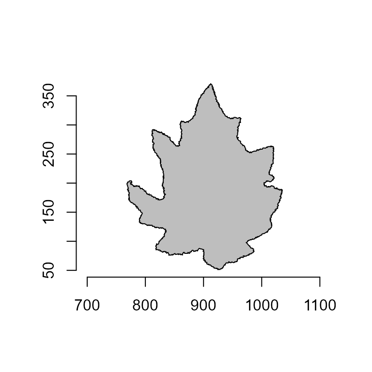
o2 <- cont[["2"]]
plot_polygon(o2)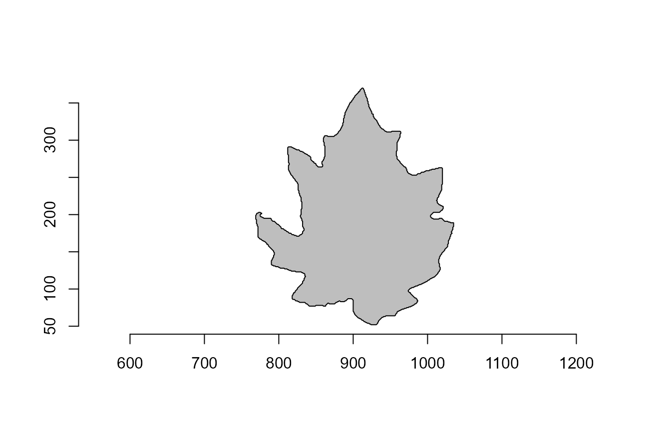
Rotate polygons
poly_rotate() can be used to rotate the polygon
coordinates by a angle (0-360 degrees) in the trigonometric
direction (anti-clockwise).
rot <- poly_rotate(o2, angle = 45)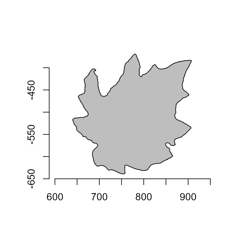
Flip polygons
poly_flip_x() and poly_flip_y() can be used
to flip shapes along the x and y axis, respectively.
flip <- list(
  fx = poly_flip_x(o2),
  fy = poly_flip_y(o2)
)
plot_polygon(flip, merge = FALSE, aspect_ratio = 1)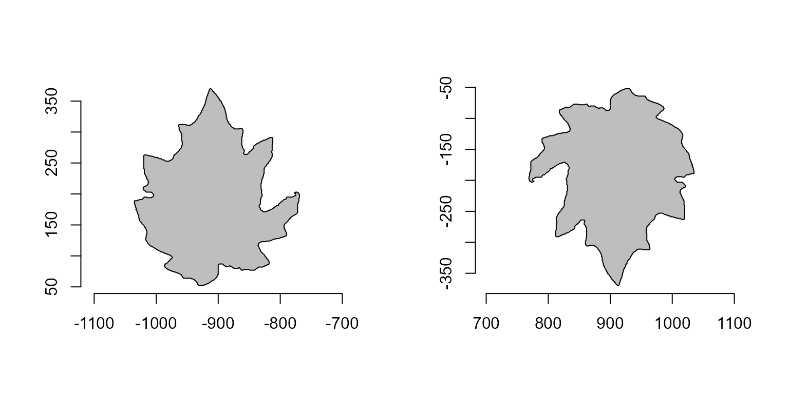
#> $fx
#> NULL
#>
#> $fy
#> NULL
Sample points
poly_sample() samples n coordinates among
existing points, and poly_sample_prop() samples a
proportion of coordinates among existing.
# sample 50 coordinates
poly_sample(o2, n = 50) |> plot_polygon()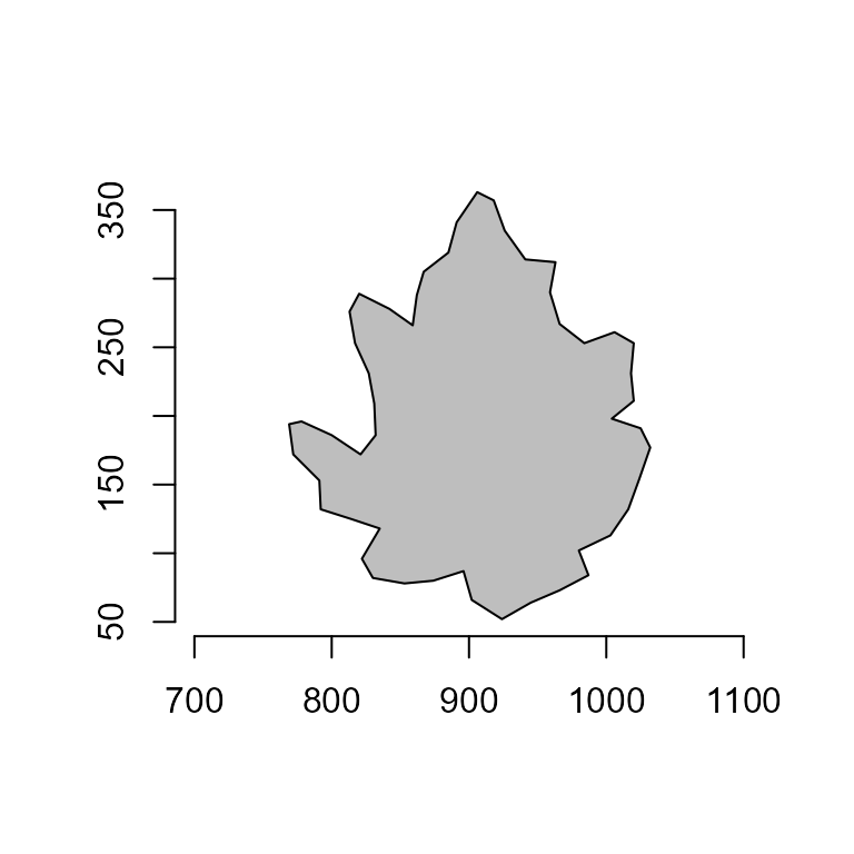
# sample 10% of the coordinates
poly_sample_prop(o2, prop = 0.1) |> plot_polygon()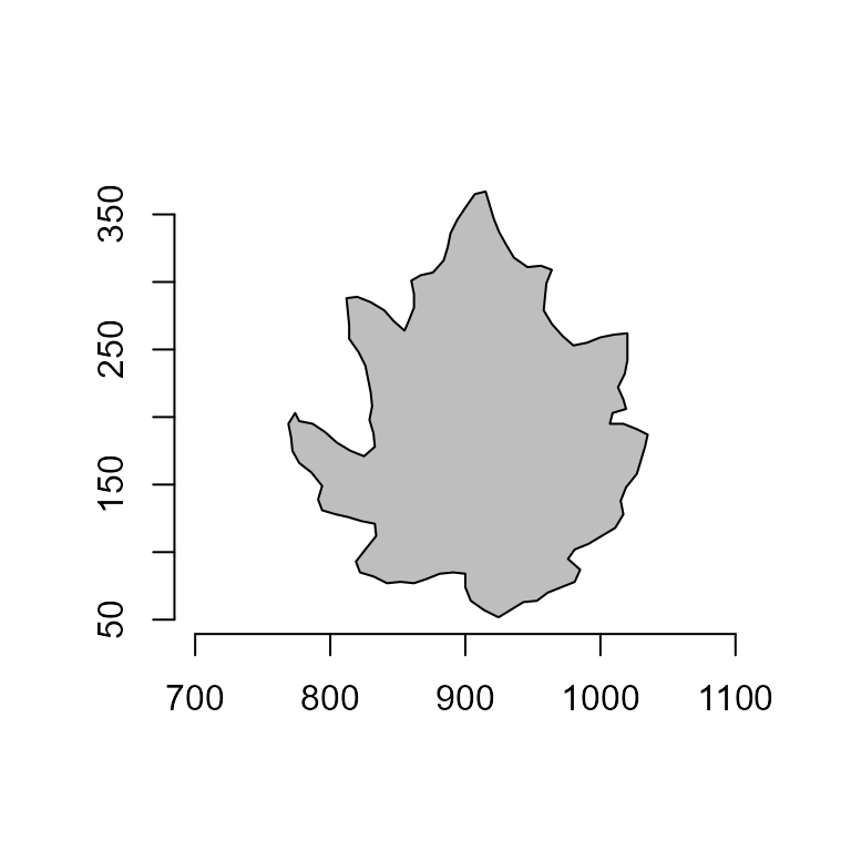
Smooth polygons
poly_smooth() smooths a polygon contour by combining
sampling prop coordinate points and interpolating them
using vertices vertices.
smooths <-
  list(
    s1 <- poly_smooth(o2, prop = 0.2, plot = FALSE),
    s2 <- poly_smooth(o2, prop = 0.1, plot = FALSE),
    s1 <- poly_smooth(o2, prop = 0.05, plot = FALSE)
  )
plot_polygon(smooths, merge = FALSE, ncol = 3)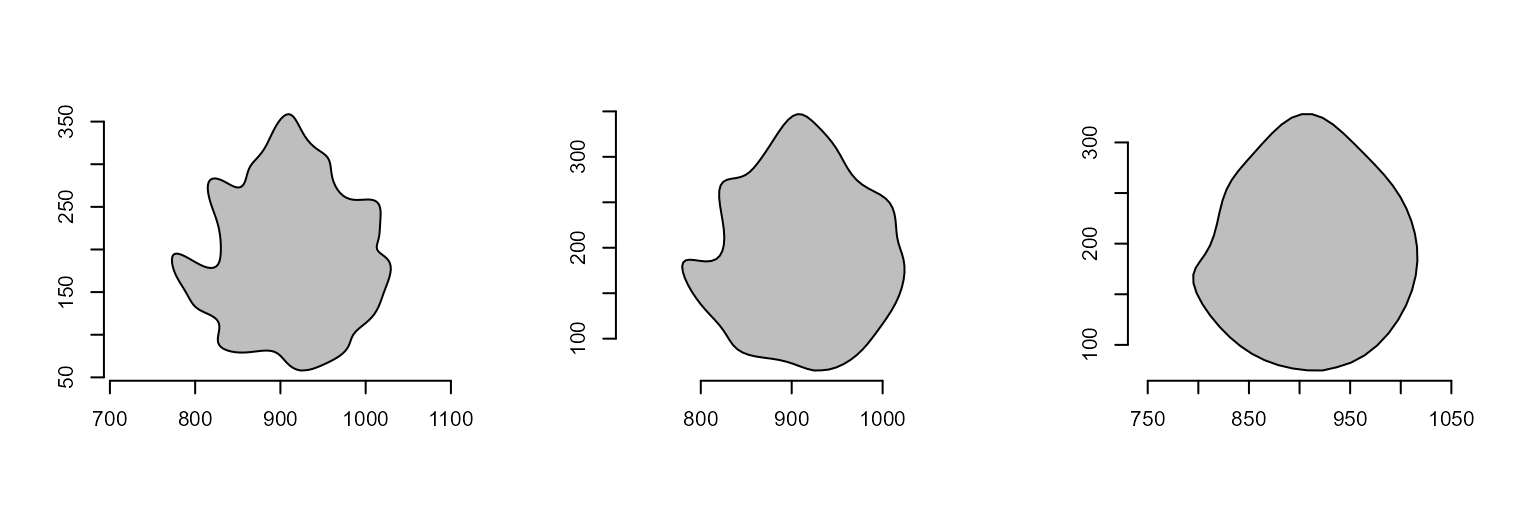
#> [[1]]
#> NULL
#>
#> [[2]]
#> NULL
#>
#> [[3]]
#> NULL
Add noise to a polygon
poly_jitter() adds a small amount of noise to a set of
point coordinates. See base::jitter() for more details.
poly_jitter(o2, noise_x = 5, noise_y = 5) |> plot_polygon()