Several useful functions for analyzing polygons. All of them are based on a set of coordinate points that describe the edge of the object(s). If a list of polygons is provided, it loops through the list and computes what is needed for each element of the list.
Polygon measures
conv_hull()Computes the convex hull of a set of points.conv_hull_unified()Computes the convex hull of a set of points. Compared toconv_hull(),conv_hull_unified()binds (unifies) the coordinates when x is a list of coordinates.poly_area()Computes the area of a polygon given by the vertices in the vectors x and y using the Shoelace formula, as follows (Lee and Lim, 2017): $$A=\frac{1}{2}\left|\sum_{i=1}^{n}\left(x_{i} y_{i+1}-x_{i+1} y_{i}\right)\right|$$ wherexandyare the coordinates that form the corners of a polygon, andnis the number of coordinates.poly_angles()Calculates the internal angles of the polygon using the law of cosines.poly_lw()Returns the length and width of a polygon based on its alignment to the y-axis (with poly_align()). The length is defined as the range along the x-axis, and the width is defined as the range on the y-axis.poly_mass()Computes the center of mass of a polygon given by the vertices in the vectors inx.poly_solidity()Computes the solidity of a shape as the ratio of the shape area and the convex hull area.
Perimeter measures
poly_slide()Slides the coordinates of a polygon given by the vertices in the vectors x and y so that the id-th point becomes the first one.poly_distpts()Computes the Euclidean distance between every point of a polygon given by the vertices in the vectors x and y.poly_centdist()Computes the Euclidean distance between every point on the perimeter and the centroid of the object.poly_perimeter()Computes the perimeter of a polygon given by the vertices in the vectors x and y.poly_caliper()Computes the caliper (also called the Feret's diameter) of a polygon given by the vertices in the vectors x and y.
Circularity measures (Montero et al. 2009).
poly_circularity()computes the circularity (C), also called shape compactness or roundness measure, of an object. It is given byC = P^2 / A, where P is the perimeter and A is the area of the object.poly_circularity_norm()computes the normalized circularity (Cn), which is unity for a circle. This measure is invariant under translation, rotation, scaling transformations, and is dimensionless. It is given by:Cn = P^2 / 4*pi*A.poly_circularity_haralick()computes Haralick's circularity (CH). The method is based on computing all Euclidean distances from the object centroid to each boundary pixel. With this set of distances, the mean (m) and the standard deviation (sd) are computed. These statistical parameters are used to calculate the circularity, CH, of a shape asCH = m/sd.poly_convexity()computes the convexity of a shape using the ratio between the perimeter of the convex hull and the perimeter of the polygon.poly_eccentricity()computes the eccentricity of a shape using the ratio of the eigenvalues (inertia axes of coordinates).poly_elongation()computes the elongation of a shape as1 - width / length.
Utilities for polygons
poly_check()Checks a set of coordinate points and returns a matrix with x and y columns.poly_is_closed()Returns a logical value indicating if a polygon is closed.poly_close()andpoly_unclose()close and unclose a polygon, respectively.poly_rotate()Rotates the polygon coordinates by an angle (0-360 degrees) in the counterclockwise direction.poly_flip_x(),poly_flip_y()flip shapes along the x-axis and y-axis, respectively.poly_align()Aligns the coordinates along their longer axis using the var-cov matrix and eigen values.poly_center()Centers the coordinates on the origin.poly_sample()Samples n coordinates from existing points. Defaults to 50.poly_sample_prop()Samples a proportion of coordinates from existing points. Defaults to 0.1.poly_spline()Interpolates the polygon contour.poly_smooth()Smooths the polygon contour using a simple moving average.poly_jitter()Adds a small amount of noise to a set of point coordinates. Seebase::jitter()for more details.
poly_measures()Is a wrapper around thepoly_*()functions.
Usage
poly_check(x)

poly_is_closed(x)

poly_close(x)

poly_unclose(x)

poly_angles(x)

poly_limits(x)

conv_hull(x)

conv_hull_unified(x)

poly_area(x)

poly_slide(x, fp = 1)

poly_distpts(x)

poly_centdist(x)

poly_perimeter(x)

poly_rotate(x, angle, plot = TRUE)

poly_align(x, plot = TRUE)

poly_center(x, plot = TRUE)

poly_lw(x)

poly_eccentricity(x)

poly_convexity(x)

poly_caliper(x)

poly_elongation(x)

poly_solidity(x)

poly_flip_y(x)

poly_flip_x(x)

poly_sample(x, n = 50)

poly_sample_prop(x, prop = 0.1)

poly_jitter(x, noise_x = 1, noise_y = 1, plot = TRUE)

poly_circularity(x)

poly_circularity_norm(x)

poly_circularity_haralick(x)

poly_mass(x)

poly_spline(x, vertices = 100, k = 2)

poly_smooth(x, niter = 10, n = NULL, prop = NULL, plot = TRUE)

poly_measures(x)
Arguments
- x
A 2-column matrix with the
xandycoordinates. Ifxis a list of vector coordinates, the function will be applied to each element usingbase::lapply()orbase::sapply().- fp
The ID of the point that will become the new first point. Defaults to 1.
- angle
The angle (0-360) to rotate the object.
- plot
Should the object be plotted? Defaults to
TRUE.- n, prop
The number and proportion of coordinates to sample from the perimeter coordinates. In
poly_smooth(), these arguments can be used to sample points from the object's perimeter before smoothing.- noise_x, noise_y
A numeric factor to define the noise added to the
xandyaxes, respectively. Seebase::jitter()for more details.- vertices
The number of spline vertices to create.
- k
The number of points to wrap around the ends to obtain a smooth periodic spline.
- niter
An integer indicating the number of smoothing iterations.
Value
conv_hull()andpoly_spline()returns a matrix withxandycoordinates for the convex hull/smooth line in clockwise order. Ifxis a list, a list of points is returned.poly_area()returns adouble, or a numeric vector ifxis a list of vector points.poly_mass()returns adata.framecontaining the coordinates for the center of mass, as well as for the maximum and minimum distance from contour to the center of mass.poly_slides(),poly_distpts(),poly_spline(),poly_close(),poly_unclose(),poly_rotate(),poly_jitter(),poly_sample(),poly_sample_prop(), andpoly_measuresreturns adata.frame.poly_perimeter(),poly_lw(),poly_eccentricity(),poly_convexity(),poly_caliper(),poly_elongation(),poly_circularity_norm(),poly_circularity_haralick()returns adouble.
References
Lee, Y., & Lim, W. (2017). Shoelace Formula: Connecting the Area of a Polygon and the Vector Cross Product. The Mathematics Teacher, 110(8), 631–636. doi:10.5951/mathteacher.110.8.0631
Montero, R. S., Bribiesca, E., Santiago, R., & Bribiesca, E. (2009). State of the Art of Compactness and Circularity Measures. International Mathematical Forum, 4(27), 1305–1335.
Chen, C.H., and P.S.P. Wang. 2005. Handbook of Pattern Recognition and Computer Vision. 3rd ed. World Scientific.
Examples
# \donttest{
library(pliman)
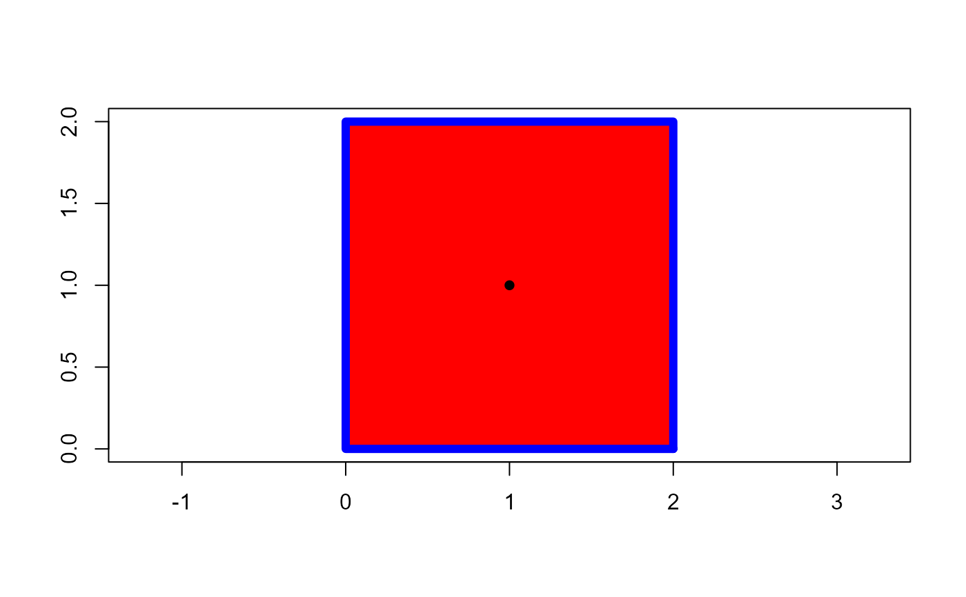
# A 2 x 2 square
df <- draw_square(side = 2)
# square area
poly_area(df)
#> [1] 4
# polygon perimeter
poly_perimeter(df)
#> [1] 6
# center of mass of the square
cm <- poly_mass(df)
plot_mass(cm)
# The convex hull will be the vertices of the square
(conv_square <- conv_hull(df) |> poly_close())
#> x y
#> 4 2 0
#> 5 0 0
#> 2 0 2
#> 3 2 2
#> 2 0
plot_contour(conv_square,
col = "blue",
lwd = 6)
 poly_area(conv_square)
#> [1] 4
################### Example with a polygon ##################
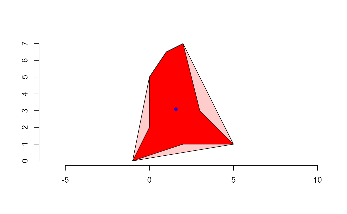
x <- c(0, 1, 2, 3, 5, 2, -1, 0, 0)
y <- c(5, 6.5, 7, 3, 1, 1, 0, 2, 5)
df_poly <- cbind(x, y)
# area of the polygon
plot_polygon(df_poly, fill = "red")
poly_area(df_poly)
#> [1] 18
# perimeter of the polygon
poly_perimeter(df_poly)
#> [1] 21.27069
# center of mass of polygon
cm <- poly_mass(df_poly)
plot_mass(cm, col = "blue")
# vertices of the convex hull
(conv_poly <- conv_hull(df_poly))
#> x y
#> [1,] 5 1.0
#> [2,] -1 0.0
#> [3,] 0 5.0
#> [4,] 1 6.5
#> [5,] 2 7.0
# area of the convex hull
poly_area(conv_poly)
#> [1] 24
plot_polygon(conv_poly,
fill = "red",
alpha = 0.2,
add = TRUE)
poly_area(conv_square)
#> [1] 4
################### Example with a polygon ##################
x <- c(0, 1, 2, 3, 5, 2, -1, 0, 0)
y <- c(5, 6.5, 7, 3, 1, 1, 0, 2, 5)
df_poly <- cbind(x, y)
# area of the polygon
plot_polygon(df_poly, fill = "red")
poly_area(df_poly)
#> [1] 18
# perimeter of the polygon
poly_perimeter(df_poly)
#> [1] 21.27069
# center of mass of polygon
cm <- poly_mass(df_poly)
plot_mass(cm, col = "blue")
# vertices of the convex hull
(conv_poly <- conv_hull(df_poly))
#> x y
#> [1,] 5 1.0
#> [2,] -1 0.0
#> [3,] 0 5.0
#> [4,] 1 6.5
#> [5,] 2 7.0
# area of the convex hull
poly_area(conv_poly)
#> [1] 24
plot_polygon(conv_poly,
fill = "red",
alpha = 0.2,
add = TRUE)
 ############ example of circularity measures ################
tri <- draw_circle(n = 200, plot = FALSE)
plot_polygon(tri, aspect_ratio = 1)
############ example of circularity measures ################
tri <- draw_circle(n = 200, plot = FALSE)
plot_polygon(tri, aspect_ratio = 1)
 poly_circularity_norm(tri)
#> [1] 0.9999169
set.seed(1)
tri2 <-
draw_circle(n = 200, plot = FALSE) |>
poly_jitter(noise_x = 100, noise_y = 100, plot = FALSE)
plot_polygon(tri2, aspect_ratio = 1)
poly_circularity_norm(tri)
#> [1] 0.9999169
set.seed(1)
tri2 <-
draw_circle(n = 200, plot = FALSE) |>
poly_jitter(noise_x = 100, noise_y = 100, plot = FALSE)
plot_polygon(tri2, aspect_ratio = 1)
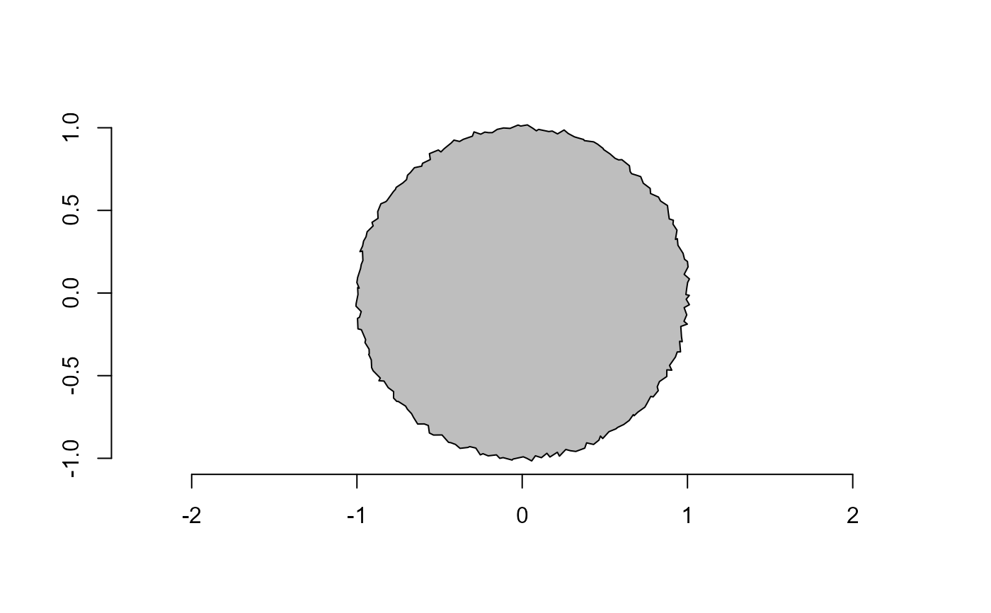 poly_circularity_norm(tri2)
#> [1] 0.7888226
# }
poly_circularity_norm(tri2)
#> [1] 0.7888226
# }