Measure leaf area using leaf images

Tiago Olivoto

2023-10-22

Getting started

We can use analyze_objects() to compute object features such as area, perimeter, radius, etc. This can be used, for example, to compute leaf area. Let’s compute the leaf area of leaves with analyze_objects(). First, we use image_segmentation() to identify candidate indexes to segment foreground (leaves) from background.

library(pliman)
#> |==========================================================|
#> | Tools for Plant Image Analysis (pliman 2.1.0)            |
#> | Author: Tiago Olivoto                                    |
#> | Type `citation('pliman')` to know how to cite pliman     |
#> | Visit 'http://bit.ly/pkg_pliman' for a complete tutorial |
#> |==========================================================|
path <- "https://raw.githubusercontent.com/TiagoOlivoto/images/master/pliman"
leaves <- 
  image_import("leaves2.jpg",
               path = path,
               plot = TRUE)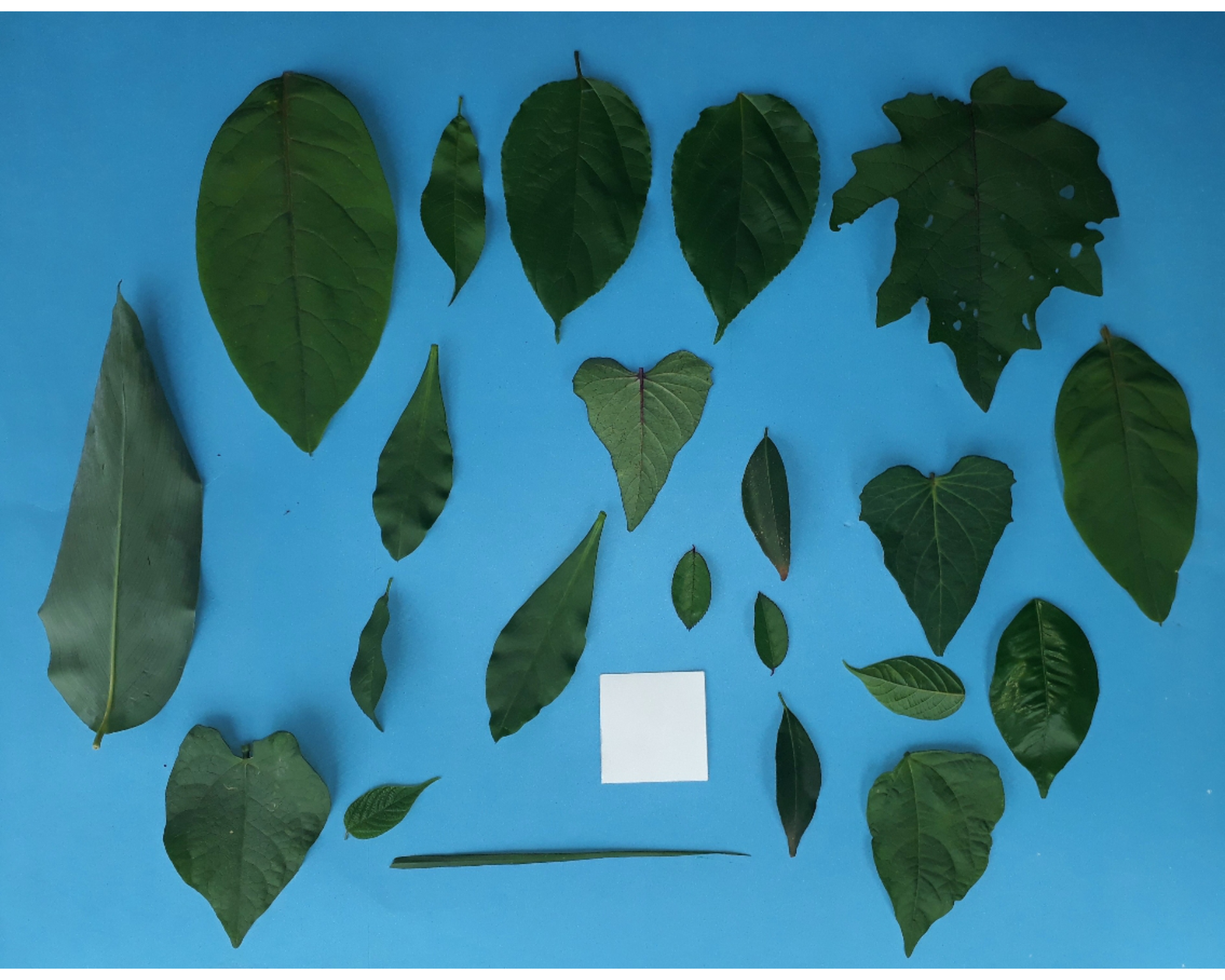

image_index(leaves)
#> Using downsample = 2 so that the number of rendered pixels approximates the `max_pixels`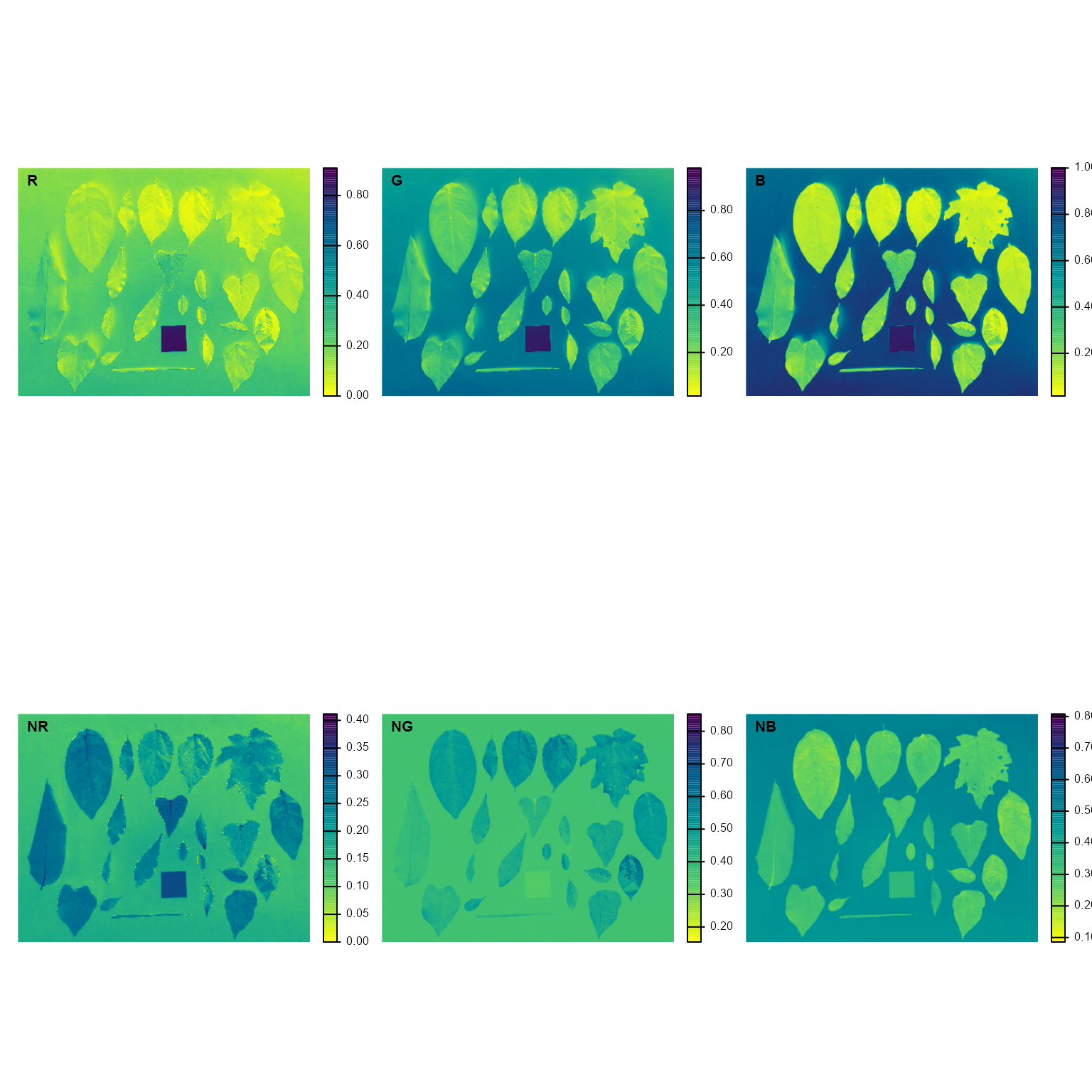

B (Blue) and NB (Normalized Blue) are two possible candidates to segment the leaves from the background. We will use the NB index here (default option in analyze_objects()). The measurement of the leaf area in this approach can be done in two main ways: 1) using an object of known area, and 2) knowing the image resolution in dpi (dots per inch).

Using an object of known area

• Count the number of objects (leaves in this case)

Here, we use the argument marker = "id" of the function analyze_objects() to obtain the identification of each object (leaf), allowing for further adjustment of the leaf area.

count <- analyze_objects(leaves, marker = "id")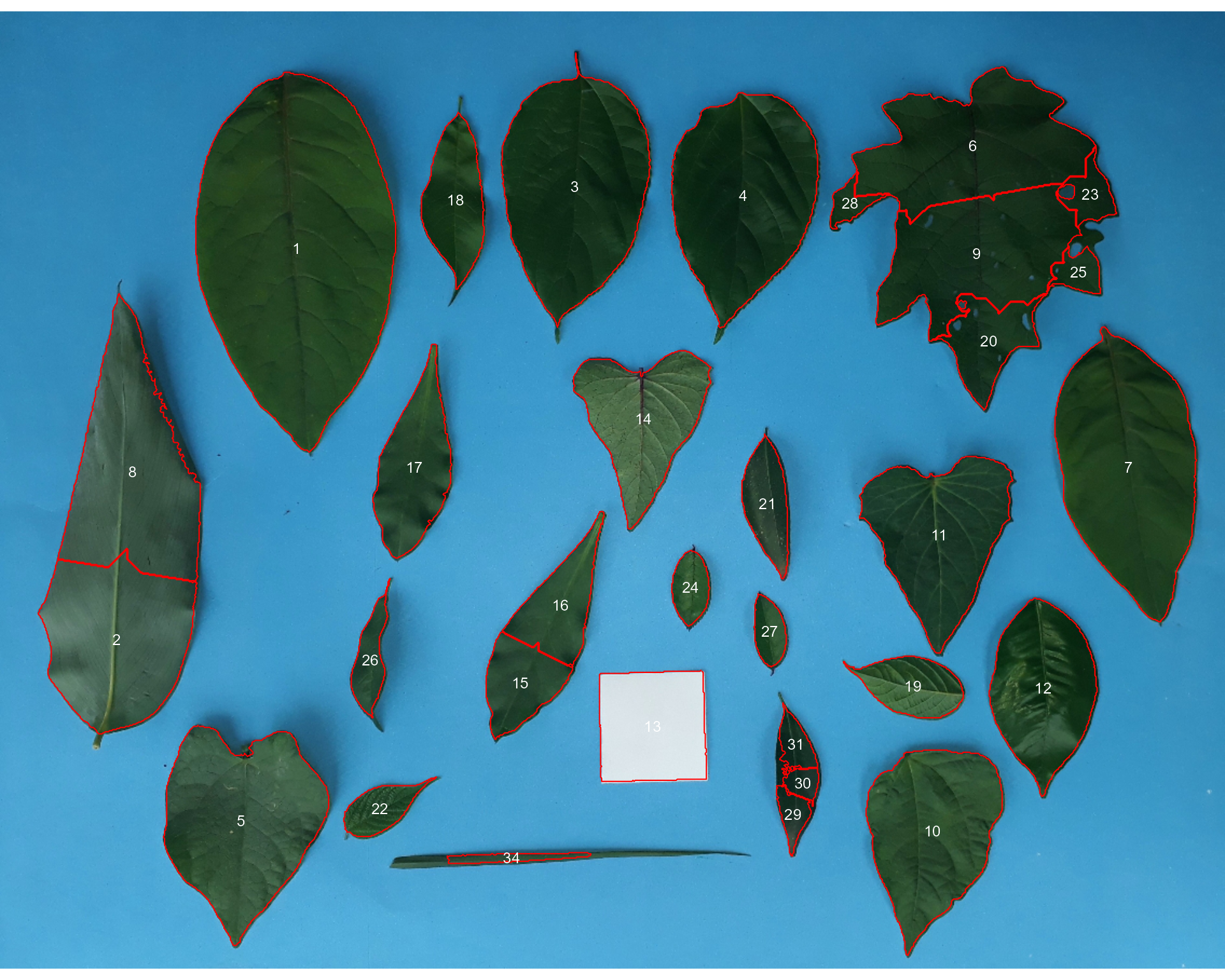

Note that “holes” in some leaves resulted in the segmentation of one leaf in more than one object (e.g., 5, 8, 22, 25, 18, 28). This will not affect the total leaf area, but the area of individual leaves and the average leaf area. This can be solved by either setting the argument fill_hull = TRUE or watershed = FALSE (To don’t implement the watershed-based object segmentation). Let’s see how much better we can go.

count <-
  analyze_objects(leaves,
                  marker = "id",
                  fill_hull = TRUE)

Almost there! Due to the morphology of the leaf composed by objects 2 and 23, it was segmented into two objects. This can be solved by setting the argument object_size = "large" that will change the default (medium) values for tolerance and extension arguments.

count <-
  analyze_objects(leaves,
                  marker = "id",
                  fill_hull = TRUE,
                  object_size = "large")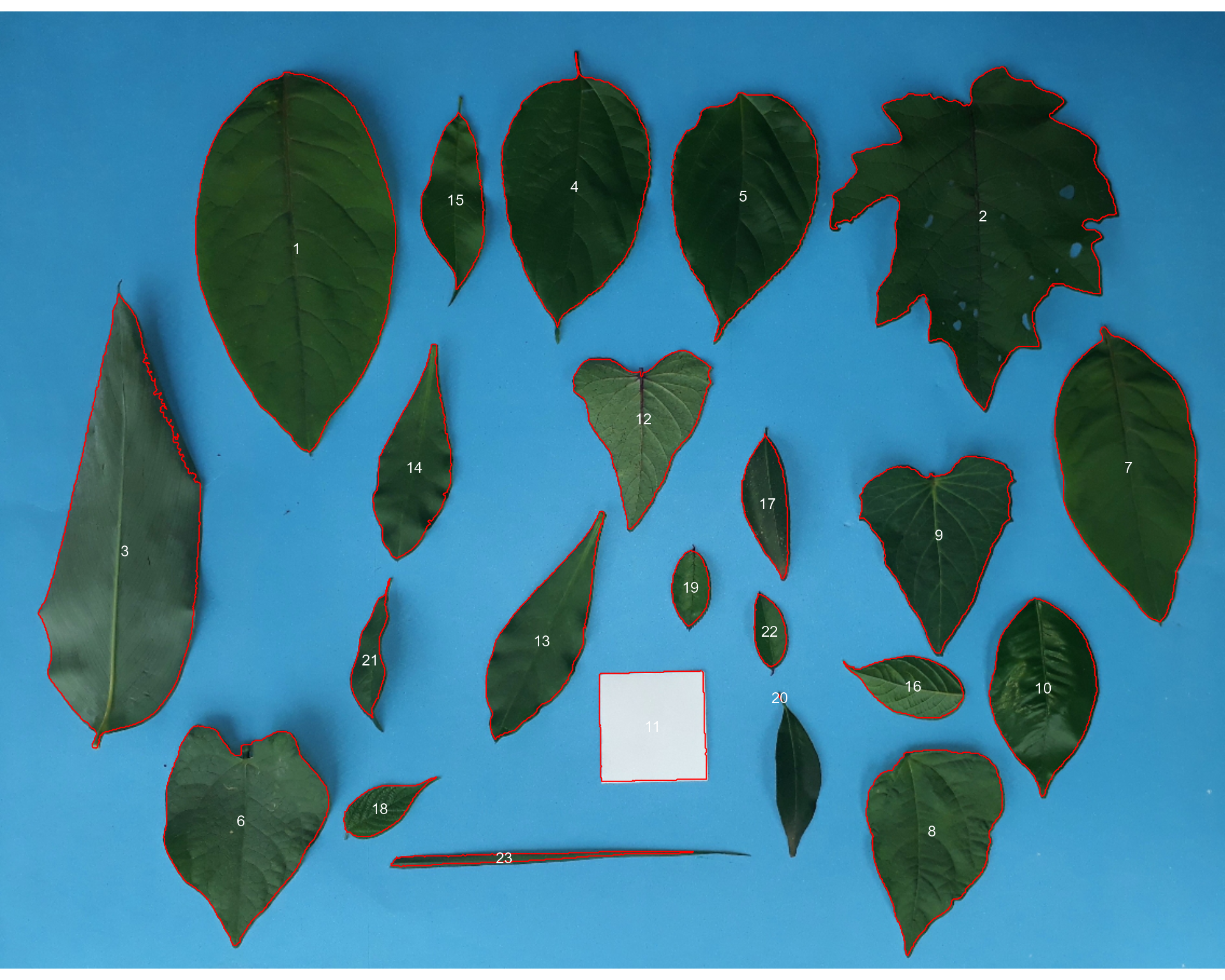

When the objects are not touching each other, the argument watershed = FALSE would be a better option.

analyze_objects(leaves,
                watershed = FALSE)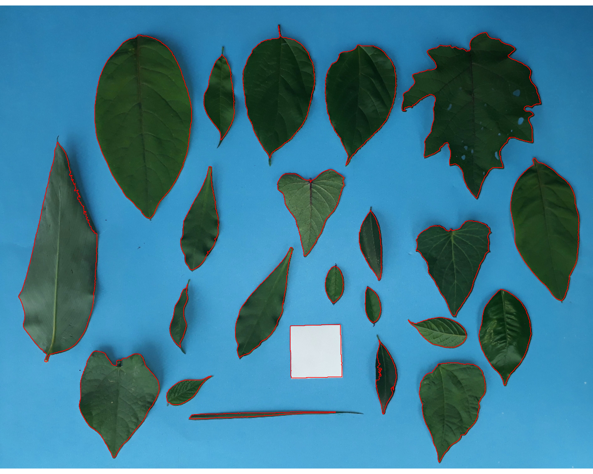

And here we are! Now, all leaves were identified correctly, but all measures were given in pixel units. The next step is to convert these measures to metric units.

• Convert the leaf area by the area of the known object

The function get_measures() is used to adjust the leaf area using object 10, a square with a side of 5 cm (25 cm\(^2\)).

area <-
  get_measures(count,
               id = 11,
               area ~ 25)
#> -----------------------------------------
#> measures corrected with:
#> object id: 11
#> area     : 25
#> -----------------------------------------
#> Total    : 801.522 
#> Average  : 36.433 
#> -----------------------------------------
# plot the area to the segmented image
image_segment(leaves, index = "NB", verbose = FALSE)
plot_measures(area,
              measure = "area",
              col = "red") # default is "white"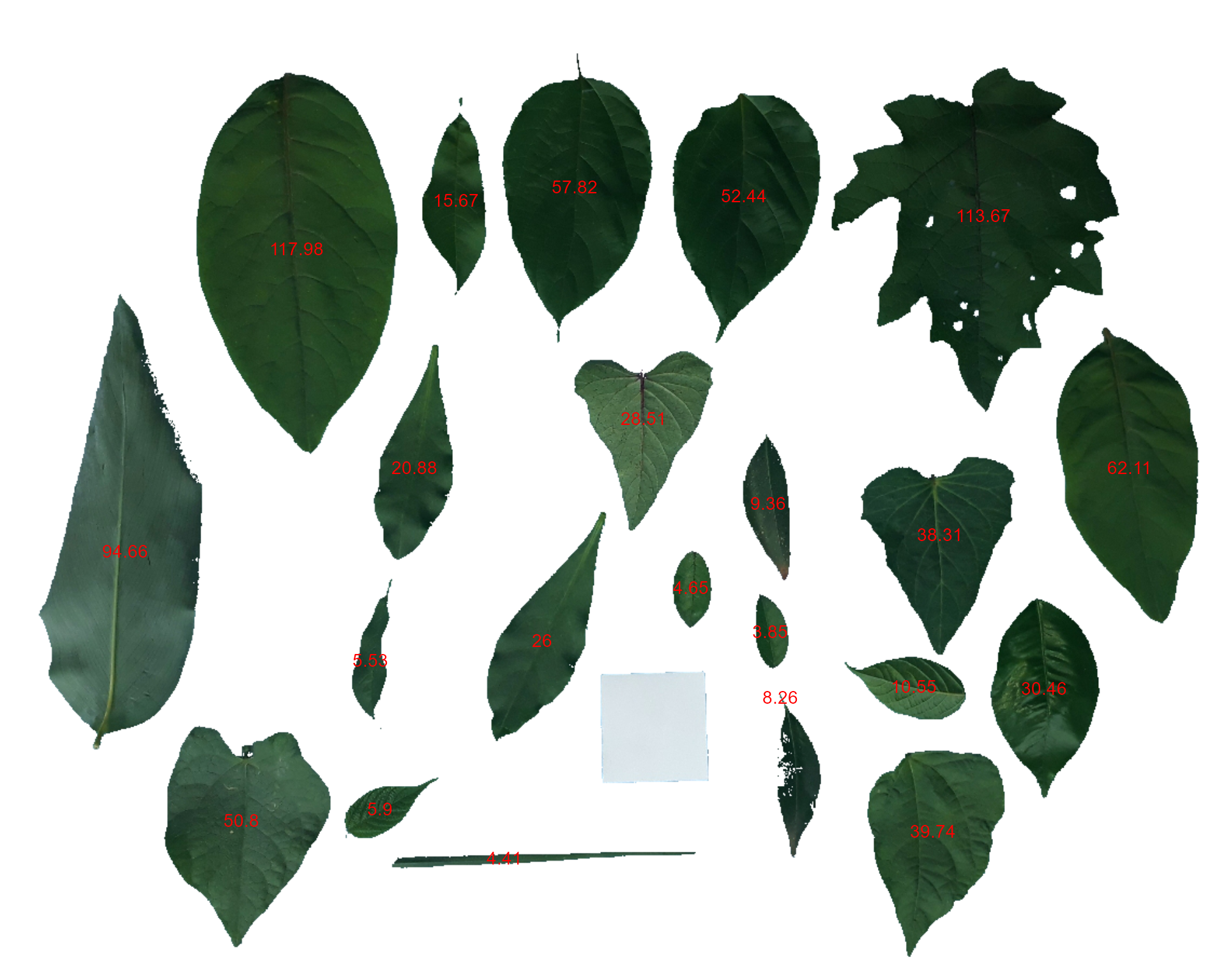

knowing the image resolution in dpi (dots per inch)

When the image resolution is known, the measures in pixels obtained with analyze_objects() are corrected by the image resolution. The function dpi() can be used to compute the dpi of an image, provided that the size of any object is known. See the dpi section for more details. In this case, the estimated resolution considering the calibration of object 10 was ~50.5 DPIs. We inform this value in the dpi argument of get_measures().

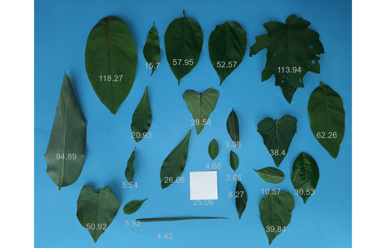
area2 <- get_measures(count, dpi = 50.5)
plot(leaves)
plot_measures(area2,
              measure = "area",
              vjust = -60,
              col = "gray") # default is "white"

A little bit more!

At this link you will find more examples on how to use {pliman} to analyze plant images. Source code and images can be downloaded here. You can also find a talk (Portuguese language) about {pliman} here. Lights, camera, {pliman}!