analyze_objects()provides tools for counting and extracting object features (e.g., area, perimeter, radius, pixel intensity) in an image. See more at the Details section.analyze_objects_iter()provides an iterative section to measure object features using an object with a known area.plot.anal_obj()produces a histogram for the R, G, and B values when argumentobject_indexis used in the functionanalyze_objects().
Usage
analyze_objects(
  img,
  foreground = NULL,
  background = NULL,
  pick_palettes = FALSE,
  segment_objects = TRUE,
  viewer = get_pliman_viewer(),
  reference = FALSE,
  reference_area = NULL,
  back_fore_index = "R/(G/B)",
  fore_ref_index = "B-R",
  reference_larger = FALSE,
  reference_smaller = FALSE,
  pattern = NULL,
  parallel = FALSE,
  workers = NULL,
  watershed = TRUE,
  veins = FALSE,
  sigma_veins = 1,
  ab_angles = FALSE,
  ab_angles_percentiles = c(0.25, 0.75),
  width_at = FALSE,
  width_at_percentiles = c(0.05, 0.25, 0.5, 0.75, 0.95),
  haralick = FALSE,
  har_nbins = 32,
  har_scales = 1,
  har_band = 1,
  pcv = FALSE,
  pcv_niter = 100,
  resize = FALSE,
  trim = FALSE,
  fill_hull = FALSE,
  filter = FALSE,
  invert = FALSE,
  object_size = "medium",
  index = "NB",
  r = 1,
  g = 2,
  b = 3,
  re = 4,
  nir = 5,
  object_index = NULL,
  pixel_level_index = FALSE,
  return_mask = FALSE,
  efourier = FALSE,
  nharm = 10,
  threshold = "Otsu",
  k = 0.1,
  windowsize = NULL,
  tolerance = NULL,
  extension = NULL,
  lower_noise = 0.1,
  lower_size = NULL,
  upper_size = NULL,
  topn_lower = NULL,
  topn_upper = NULL,
  lower_eccent = NULL,
  upper_eccent = NULL,
  lower_circ = NULL,
  upper_circ = NULL,
  randomize = TRUE,
  nrows = 1000,
  plot = TRUE,
  show_original = TRUE,
  show_chull = FALSE,
  show_contour = TRUE,
  contour_col = "red",
  contour_size = 1,
  show_lw = FALSE,
  show_background = TRUE,
  show_segmentation = FALSE,
  col_foreground = NULL,
  col_background = NULL,
  marker = FALSE,
  marker_col = NULL,
  marker_size = NULL,
  save_image = FALSE,
  prefix = "proc_",
  dir_original = NULL,
  dir_processed = NULL,
  verbose = TRUE
)

# S3 method for anal_obj
plot(
  x,
  which = "measure",
  measure = "area",
  type = c("density", "histogram"),
  ...
)

analyze_objects_iter(pattern, known_area, verbose = TRUE, ...)
Arguments
- img
The image to be analyzed.
- foreground, background
A color palette for the foregrond and background, respectively (optional). If a chacarceter is used (eg.,
foreground = "fore"), the function will search in the current working directory a valid image named "fore".- pick_palettes
Logical argument indicating wheater the user needs to pick up the color palettes for foreground and background for the image. If
TRUEpick_palette()will be called internally so that the user can sample color points representing foreground and background.- segment_objects
Segment objects in the image? Defaults to
TRUE. In this case, objects are segmented using the index defined in theindexargument, and each object is analyzed individually. Ifsegment_objects = FALSEis used, the objects are not segmented and the entire image is analyzed. This is useful, for example, when analyzing an image without background, where anobject_indexcould be computed for the entire image, like the index of a crop canopy.- viewer
The viewer option. This option controls the type of viewer to use for interactive plotting (eg., when
pick_palettes = TRUE). If not provided, the value is retrieved usingget_pliman_viewer().- reference
Logical to indicate if a reference object is present in the image. This is useful to adjust measures when images are not obtained with standard resolution (e.g., field images). See more in the details section.
- reference_area
The known area of the reference objects. The measures of all the objects in the image will be corrected using the same unit of the area informed here.
- back_fore_index
A character value to indicate the index to segment the foreground (objects and reference) from the background. Defaults to
"R/(G/B)". This index is optimized to segment white backgrounds from green leaves and a blue reference object.- fore_ref_index
A character value to indicate the index to segment objects and the reference object. It can be either an available index in
pliman(seepliman_indexes()or an own index computed with the R, G, and B bands. Defaults to"B-R". This index is optimized to segment green leaves from a blue reference object after a white background has been removed.- reference_larger, reference_smaller
Logical argument indicating when the larger/smaller object in the image must be used as the reference object. This only is valid when
referenceis set toTRUEandreference_areaindicates the area of the reference object. IMPORTANT. Whenreference_smalleris used, objects with an area smaller than 1% of the mean of all the objects are ignored. This is used to remove possible noise in the image such as dust. So, be sure the reference object has an area that will be not removed by that cutpoint.- pattern
A pattern of file name used to identify images to be imported. For example, if
pattern = "im"all images in the current working directory that the name matches the pattern (e.g., img1.-, image1.-, im2.-) will be imported as a list. Providing any number as pattern (e.g.,pattern = "1") will select images that are named as 1.-, 2.-, and so on. An error will be returned if the pattern matches any file that is not supported (e.g., img1.pdf).- parallel
If
TRUEprocesses the images asynchronously (in parallel) in separate R sessions running in the background on the same machine. It may speed up the processing time, especially whenpatternis used is informed. Whenobject_indexis informed, multiple sections will be used to extract the RGB values for each object in the image. This may significantly speed up processing time when an image has lots of objects (say >1000).- workers
A positive numeric scalar or a function specifying the number of parallel processes that can be active at the same time. By default, the number of sections is set up to 30% of available cores.
- watershed
If
TRUE(default) performs watershed-based object detection. This will detect objects even when they are touching one other. IfFALSE, all pixels for each connected set of foreground pixels are set to a unique object. This is faster but is not able to segment touching objects.- veins
Logical argument indicating whether vein features are computed. This will call
object_edge()and applies the Sobel-Feldman Operator to detect edges. The result is the proportion of edges in relation to the entire area of the object(s) in the image. Note that THIS WILL BE AN OPERATION ON AN IMAGE LEVEL, NOT OBJECT!.- sigma_veins
Gaussian kernel standard deviation used in the gaussian blur in the edge detection algorithm
- ab_angles
Logical argument indicating whether apex and base angles should be computed. Defaults to
FALSE. IfTRUE,poly_apex_base_angle()are called and the base and apex angles are computed considering the 25th and 75th percentiles of the object height. These percentiles can be changed with the argumentab_angles_percentiles.- ab_angles_percentiles
The percentiles indicating the heights of the object for which the angle should be computed (from the apex and the bottom). Defaults to c(0.25, 0.75), which means considering the 25th and 75th percentiles of the object height.
- width_at
Logical. If
TRUE, the widths of the object at a given set of quantiles of the height are computed.- width_at_percentiles
A vector of heights along the vertical axis of the object at which the width will be computed. The default value is c(0.05, 0.25, 0.5, 0.75, 0.95), which means the function will return the width at the 5th, 25th, 50th, 75th, and 95th percentiles of the object's height.
- haralick
Logical value indicating whether Haralick features are computed. Defaults to
FALSE.- har_nbins
An integer indicating the number of bins using to compute the Haralick matrix. Defaults to 32. See Details
- har_scales
A integer vector indicating the number of scales to use to compute the Haralick features. See Details.
- har_band
The band to compute the Haralick features (1 = R, 2 = G, 3 = B). Defaults to 1.
- pcv
Computes the Perimeter Complexity Value? Defaults to
FALSE.- pcv_niter
An integer specifying the number of smoothing iterations for computing the Perimeter Complexity Value. Defaults to 100.
- resize
Resize the image before processing? Defaults to
FALSE. Use a numeric value of range 0-100 (proportion of the size of the original image).- trim
Number of pixels removed from edges in the analysis. The edges of images are often shaded, which can affect image analysis. The edges of images can be removed by specifying the number of pixels. Defaults to
FALSE(no trimmed edges).- fill_hull
Fill holes in the binary image? Defaults to
FALSE. This is useful to fill holes in objects that have portions with a color similar to the background. IMPORTANT: Objects touching each other can be combined into one single object, which may underestimate the number of objects in an image.- filter
Performs median filtering in the binary image? See more at
image_filter(). Defaults toFALSE. Use a positive integer to define the size of the median filtering. Larger values are effective at removing noise, but adversely affect edges.- invert
Inverts the binary image if desired. This is useful to process images with a black background. Defaults to
FALSE. Ifreference = TRUEis use,invertcan be declared as a logical vector of length 2 (eg.,invert = c(FALSE, TRUE). In this case, the segmentation of objects and reference from the foreground usingback_fore_indexis performed using the default (not inverted), and the segmentation of objects from the reference is performed by inverting the selection (selecting pixels higher than the threshold).- object_size
The size of the object. Used to automatically set up
toleranceandextensionparameters. One of the following."small"(e.g, wheat grains),"medium"(e.g, soybean grains),"large"(e.g, peanut grains), and"elarge"(e.g, soybean pods)`.- index
A character value specifying the target mode for conversion to binary image when
foregroundandbackgroundare not declared. Defaults to"NB"(normalized blue). Seeimage_index()for more details. User can also calculate your own index using the bands names, e.g.index = "R+B/G"- r, g, b, re, nir
The red, green, blue, red-edge, and near-infrared bands of the image, respectively. Defaults to 1, 2, 3, 4, and 5, respectively. If a multispectral image is provided (5 bands), check the order of bands, which are frequently presented in the 'BGR' format.
- object_index
Defaults to
FALSE. If an index is informed, the average value for each object is returned. It can be the R, G, and B values or any operation involving them, e.g.,object_index = "R/B". In this case, it will return for each object in the image, the average value of the R/B ratio. Usepliman_indexes_eq()to see the equations of available indexes.- pixel_level_index
Return the indexes computed in
object_indexin the pixel level? Defaults toFALSEto avoid returning large data.frames.- return_mask
Returns the mask for the analyzed image? Defaults to
FALSE.- efourier
Logical argument indicating if Elliptical Fourier should be computed for each object. This will call
efourier()internally. Itefourier = TRUEis used, both standard and normalized Fourier coefficients are returned.- nharm
An integer indicating the number of harmonics to use. Defaults to 10. For more details see
efourier().- threshold
The theshold method to be used.
By default (
threshold = "Otsu"), a threshold value based on Otsu's method is used to reduce the grayscale image to a binary image. If a numeric value is informed, this value will be used as a threshold.If
threshold = "adaptive", adaptive thresholding (Shafait et al. 2008) is used, and will depend on thekandwindowsizearguments.If any non-numeric value different than
"Otsu"and"adaptive"is used, an iterative section will allow you to choose the threshold based on a raster plot showing pixel intensity of the index.
- k
a numeric in the range 0-1. when
kis high, local threshold values tend to be lower. whenkis low, local threshold value tend to be higher.- windowsize
windowsize controls the number of local neighborhood in adaptive thresholding. By default it is set to
1/3 * minxy, whereminxyis the minimum dimension of the image (in pixels).- tolerance
The minimum height of the object in the units of image intensity between its highest point (seed) and the point where it contacts another object (checked for every contact pixel). If the height is smaller than the tolerance, the object will be combined with one of its neighbors, which is the highest.
- extension
Radius of the neighborhood in pixels for the detection of neighboring objects. Higher value smooths out small objects.
- lower_noise
To prevent noise from affecting the image analysis, objects with lesser than 10% of the mean area of all objects are removed (
lower_noise = 0.1). Increasing this value will remove larger noises (such as dust points), but can remove desired objects too. To define an explicit lower or upper size, use thelower_sizeandupper_sizearguments.- lower_size, upper_size
Lower and upper limits for size for the image analysis. Plant images often contain dirt and dust. Upper limit is set to
NULL, i.e., no upper limit used. One can set a known area or uselower_limit = 0to select all objects (not advised). Objects that matches the size of a given range of sizes can be selected by setting up the two arguments. For example, iflower_size = 120andupper_size = 140, objects with size greater than or equal 120 and less than or equal 140 will be considered.- topn_lower, topn_upper
Select the top
nobjects based on its area.topn_lowerselects thenelements with the smallest area whereastopn_upperselects thenobjects with the largest area.- lower_eccent, upper_eccent, lower_circ, upper_circ
Lower and upper limit for object eccentricity/circularity for the image analysis. Users may use these arguments to remove objects such as square papers for scale (low eccentricity) or cut petioles (high eccentricity) from the images. Defaults to
NULL(i.e., no lower and upper limits).- randomize
Randomize the lines before training the model?
- nrows
The number of lines to be used in training step. Defaults to 2000.
- plot
Show image after processing?
- show_original
Show the count objects in the original image?
- show_chull
Show the convex hull around the objects? Defaults to
FALSE.- show_contour
Show a contour line around the objects? Defaults to
TRUE.- contour_col, contour_size
The color and size for the contour line around objects. Defaults to
contour_col = "red"andcontour_size = 1.- show_lw
If
TRUE, plots the length and width lines on each object callingplot_lw().- show_background
Show the background? Defaults to
TRUE. A white background is shown by default whenshow_original = FALSE.- show_segmentation
Shows the object segmentation colored with random permutations. Defaults to
FALSE.- col_foreground, col_background
Foreground and background color after image processing. Defaults to
NULL, in which"black", and"white"are used, respectively.- marker, marker_col, marker_size
The type, color and size of the object marker. Defaults to
NULL, which plots the object id. Usemarker = "point"to show a point in each object ormarker = FALSEto omit object marker.- save_image
Save the image after processing? The image is saved in the current working directory named as
proc_*where*is the image name given inimg.- prefix
The prefix to be included in the processed images. Defaults to
"proc_".- dir_original, dir_processed
The directory containing the original and processed images. Defaults to
NULL. In this case, the function will search for the imageimgin the current working directory. After processing, whensave_image = TRUE, the processed image will be also saved in such a directory. It can be either a full path, e.g.,"C:/Desktop/imgs", or a subfolder within the current working directory, e.g.,"/imgs".- verbose
If
TRUE(default) a summary is shown in the console.- x
An object of class
anal_obj.- which
Which to plot. Either 'measure' (object measures) or 'index' (object index). Defaults to
"measure".- measure
The measure to plot. Defaults to
"area".- type
The type of plot. Either
"hist"or"density". Partial matches are recognized.- ...
Depends on the function:
For
analyze_objects_iter(), further arguments passed on toanalyze_objects().
- known_area
The known area of the template object.
Value
analyze_objects() returns a list with the following objects:
resultsA data frame with the following variables for each object in the image:id: object identification.x,y: x and y coordinates for the center of mass of the object.area: area of the object (in pixels).area_ch: the area of the convex hull around object (in pixels).perimeter: perimeter (in pixels).radius_min,radius_mean, andradius_max: The minimum, mean, and maximum radius (in pixels), respectively.radius_sd: standard deviation of the mean radius (in pixels).diam_min,diam_mean, anddiam_max: The minimum, mean, and maximum diameter (in pixels), respectively.major_axis,minor_axis: elliptical fit for major and minor axes (in pixels).caliper: The longest distance between any two points on the margin of the object. Seepoly_caliper()for more detailslength,widthThe length and width of objects (in pixels). These measures are obtained as the range of x and y coordinates after aligning each object withpoly_align().radius_ratio: radius ratio given byradius_max / radius_min.theta: object angle (in radians).eccentricity: elliptical eccentricity computed using the ratio of the eigen values (inertia axes of coordinates).form_factor(Wu et al., 2007): the difference between a leaf and a circle. It is defined as4*pi*A/P, where A is the area and P is the perimeter of the object.narrow_factor(Wu et al., 2007): Narrow factor (caliper / length).asp_ratio(Wu et al., 2007): Aspect ratio (length / width).rectangularity(Wu et al., 2007): The similarity between a leaf and a rectangle (length * width/ area).pd_ratio(Wu et al., 2007): Ratio of perimeter to diameter (perimeter / caliper)plw_ratio(Wu et al., 2007): Perimeter ratio of length and width (perimeter / (length + width))solidity: object solidity given byarea / area_ch.convexity: The convexity of the object computed using the ratio between the perimeter of the convex hull and the perimeter of the polygon.elongation: The elongation of the object computed as1 - width / length.circularity: The object circularity given byperimeter ^ 2 / area.circularity_haralick: The Haralick's circularity (CH), computed asCH = m/sd, wheremandsdare the mean and standard deviations from each pixels of the perimeter to the centroid of the object.circularity_norm: The normalized circularity (Cn), to be unity for a circle. This measure is computed asCn = perimeter ^ 2 / 4*pi*areaand is invariant under translation, rotation, scaling transformations, and dimensionless.asm: The angular second-moment feature.con: The contrast featurecor: Correlation measures the linear dependency of gray levels of neighboring pixels.var: The variance of gray levels pixels.idm: The Inverse Difference Moment (IDM), i.e., the local homogeneity.sav: The Sum Average.sva: The Sum Variance.sen: Sum Entropy.dva: Difference Variance.den: Difference Entropyf12: Difference Variance.f13: The angular second-moment feature.
statistics: A data frame with the summary statistics for the area of the objects.count: Ifpatternis used, shows the number of objects in each image.obj_rgb: Ifobject_indexis used, returns the R, G, and B values for each pixel of each object.object_index: Ifobject_indexis used, returns the index computed for each object.Elliptical Fourier Analysis: If
efourier = TRUEis used, the following objects are returned.efourier: The Fourier coefficients. For more details seeefourier().efourier_norm: The normalized Fourier coefficients. For more details seeefourier_norm().efourier_error: The error between original data and reconstructed outline. For more details seeefourier_error().efourier_power: The spectrum of harmonic Fourier power. For more details seeefourier_power().
veins: Ifveins = TRUEis used, returns, for each image, the proportion of veins (in fact the object edges) related to the total object(s)' area.analyze_objects_iter()returns a data.frame containing the features described in theresultsobject ofanalyze_objects().plot.anal_obj()returns atrellisobject containing the distribution of the pixels, optionally for each object whenfacet = TRUEis used.
Details
A binary image is first generated to segment the foreground and
background. The argument index is useful to choose a proper index to
segment the image (see image_binary() for more details). It is also
possible to provide color palettes for background and foreground (arguments
background and foreground, respectively). When this is used, a general
linear model (binomial family) fitted to the RGB values to segment fore- and
background.
Then, the number of objects in the foreground is counted. By setting up
arguments such as lower_size and upper_size, it is possible to set a
threshold for lower and upper sizes of the objects, respectively. The
argument object_size can be used to set up pre-defined values of
tolerance and extension depending on the image resolution. This will
influence the watershed-based object segmentation. Users can also tune up
tolerance and extension explicitly for a better precision of watershed
segmentation.
If watershed = FALSE is used, all pixels for each connected set of
foreground pixels in img are set to a unique object. This is faster,
especially for a large number of objects, but it is not able to segment
touching objects.
There are some ways to correct the measures based on a reference object. If
a reference object with a known area (reference_area) is used in the image
and reference = TRUE is used, the measures of the objects will be
corrected, considering the unit of measure informed in reference_area.
There are two main ways to work with reference objects.
The first, is to provide a reference object that has a contrasting color with both the background and object of interest. In this case, the arguments
back_fore_indexandfore_ref_indexcan be used to define an index to first segment the reference object and objects to be measured from the background, then the reference object from objects to be measured.The second one is to use a reference object that has a similar color to the objects to be measured, but has a contrasting size. For example, if we are counting small brown grains, we can use a brown reference template that has an area larger (says 3 times the area of the grains) and then uses
reference_larger = TRUE. With this, the larger object in the image will be used as the reference object. This is particularly useful when images are captured with background light, such as the example 2. Some types: (i) It is suggested that the reference object is not too much larger than the objects of interest (mainly when thewatershed = TRUE). In some cases, the reference object can be broken into several pieces due to the watershed algorithm. (ii) Since the reference object will increase the mean area of the object, the argumentlower_noisecan be increased. By default (lower_noise = 0.1) objects with lesser than 10% of the mean area of all objects are removed. Since the mean area will be increased, increasinglower_noisewill remove dust and noises more reliably. The argumentreference_smallercan be used in the same way
By using pattern, it is possible to process several images with common
pattern names that are stored in the current working directory or in the
subdirectory informed in dir_original. To speed up the computation time,
one can set parallel = TRUE.
analyze_objects_iter() can be used to process several images using an
object with a known area as a template. In this case, all the images in the
current working directory that match the pattern will be processed. For
each image, the function will compute the features for the objects and show
the identification (id) of each object. The user only needs to inform which
is the id of the known object. Then, given the known_area, all the
measures will be adjusted. In the end, a data.frame with the adjusted
measures will be returned. This is useful when the images are taken at
different heights. In such cases, the image resolution cannot be conserved.
Consequently, the measures cannot be adjusted using the argument dpi from
get_measures(), since each image will have a different resolution. NOTE:
This will only work in an interactive section.
Additional measures: By default, some measures are not computed, mainly due to computational efficiency when the user only needs simple measures such as area, length, and width.
If
haralick = TRUE, The function computes 13 Haralick texture features for each object based on a gray-level co-occurrence matrix (Haralick et al. 1979). Haralick features depend on the configuration of the parametershar_nbinsandhar_scales.har_nbinscontrols the number of bins used to compute the Haralick matrix. A smallerhar_nbinscan give more accurate estimates of the correlation because the number of events per bin is higher. While a higher value will give more sensitivity.har_scalescontrols the number of scales used to compute the Haralick features. Since Haralick features compute the correlation of intensities of neighboring pixels it is possible to identify textures with different scales, e.g., a texture that is repeated every two pixels or 10 pixels. By default, the Haralick features are computed with the R band. To chance this default, use the argumenthar_band. For example,har_band = 2will compute the features with the green band.If
efourier = TRUEis used, an Elliptical Fourier Analysis (Kuhl and Giardina, 1982) is computed for each object contour usingefourier().If
veins = TRUE(experimental), vein features are computed. This will callobject_edge()and applies the Sobel-Feldman Operator to detect edges. The result is the proportion of edges in relation to the entire area of the object(s) in the image. Note that THIS WILL BE AN OPERATION ON AN IMAGE LEVEL, NOT an OBJECT LEVEL! So, If vein features need to be computed for leaves, it is strongly suggested to use one leaf per image.If
ab_angles = TRUEthe apex and base angles of each object are computed withpoly_apex_base_angle(). By default, the function computes the angle from the first pixel of the apex of the object to the two pixels that slice the object at the 25th percentile of the object height (apex angle). The base angle is computed in the same way but from the first base pixel.If
width_at = TRUE, the width at the 5th, 25th, 50th, 75th, and 95th percentiles of the object height are computed by default. These quantiles can be adjusted with thewidth_at_percentilesargument.
References
Claude, J. (2008) Morphometrics with R, Use R! series, Springer 316 pp.
Gupta, S., Rosenthal, D. M., Stinchcombe, J. R., & Baucom, R. S. (2020). The remarkable morphological diversity of leaf shape in sweet potato (Ipomoea batatas): the influence of genetics, environment, and G×E. New Phytologist, 225(5), 2183–2195. doi:10.1111/NPH.16286
Haralick, R.M., K. Shanmugam, and I. Dinstein. 1973. Textural Features for Image Classification. IEEE Transactions on Systems, Man, and Cybernetics SMC-3(6): 610–621. doi:10.1109/TSMC.1973.4309314
Kuhl, F. P., and Giardina, C. R. (1982). Elliptic Fourier features of a closed contour. Computer Graphics and Image Processing 18, 236–258. doi: doi:10.1016/0146-664X(82)90034-X
Lee, Y., & Lim, W. (2017). Shoelace Formula: Connecting the Area of a Polygon and the Vector Cross Product. The Mathematics Teacher, 110(8), 631–636. doi:10.5951/mathteacher.110.8.0631
Montero, R. S., Bribiesca, E., Santiago, R., & Bribiesca, E. (2009). State of the Art of Compactness and Circularity Measures. International Mathematical Forum, 4(27), 1305–1335.
Chen, C.H., and P.S.P. Wang. 2005. Handbook of Pattern Recognition and Computer Vision. 3rd ed. World Scientific.
Wu, S. G., Bao, F. S., Xu, E. Y., Wang, Y.-X., Chang, Y.-F., and Xiang, Q.-L. (2007). A Leaf Recognition Algorithm for Plant Classification Using Probabilistic Neural Network. in 2007 IEEE International Symposium on Signal Processing and Information Technology, 11–16. doi:10.1109/ISSPIT.2007.4458016
Author
Tiago Olivoto tiagoolivoto@gmail.com
Examples
# \donttest{
library(pliman)
img <- image_pliman("soybean_touch.jpg")
obj <- analyze_objects(img)
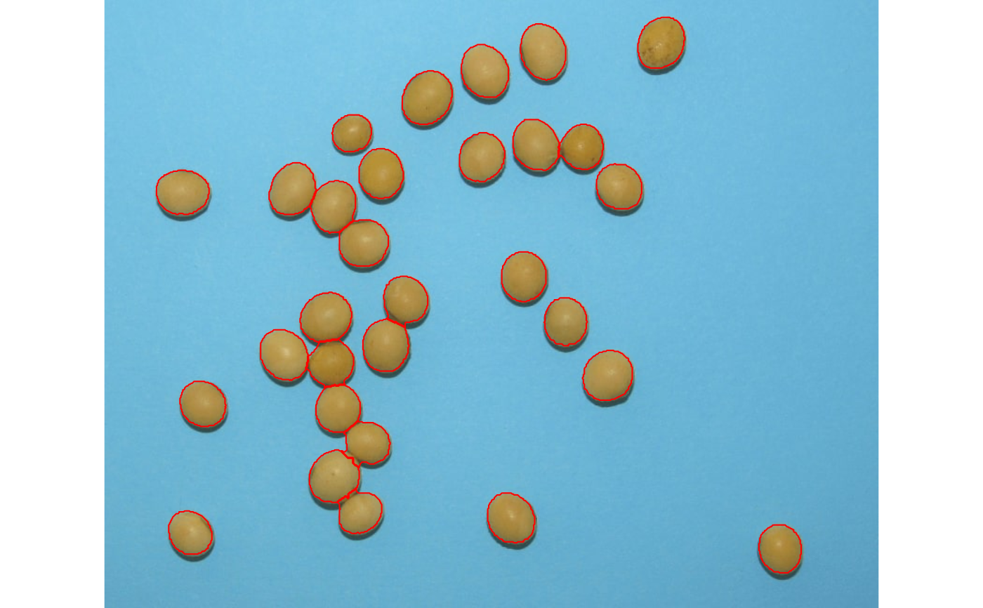 obj$statistics
#> stat value
#> 1 n 3.000000e+01
#> 2 min_area 1.366000e+03
#> 3 mean_area 2.051300e+03
#> 4 max_area 2.436000e+03
#> 5 sd_area 2.300703e+02
#> 6 sum_area 6.153900e+04
#> 7 coverage 1.151122e-01
########################### Example 1 #########################
# Enumerate the objects in the original image
# Return the top-5 grains with the largest area
top <-
analyze_objects(img,
marker = "id",
topn_upper = 5)
obj$statistics
#> stat value
#> 1 n 3.000000e+01
#> 2 min_area 1.366000e+03
#> 3 mean_area 2.051300e+03
#> 4 max_area 2.436000e+03
#> 5 sd_area 2.300703e+02
#> 6 sum_area 6.153900e+04
#> 7 coverage 1.151122e-01
########################### Example 1 #########################
# Enumerate the objects in the original image
# Return the top-5 grains with the largest area
top <-
analyze_objects(img,
marker = "id",
topn_upper = 5)
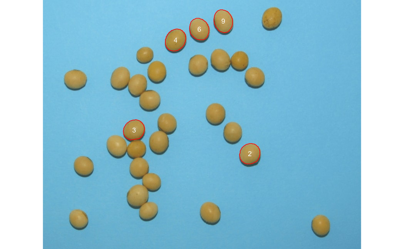 top$results
#> id x y area area_ch perimeter radius_mean radius_min
#> 4 4 344.3132 104.74372 2436 2408.0 185.6102 27.45204 24.31796
#> 9 9 468.0383 55.44180 2311 2278.0 181.0244 26.77622 23.16169
#> 3 3 236.6572 338.80546 2310 2288.5 181.0244 26.69273 23.99117
#> 6 6 405.9755 76.41826 2297 2264.5 178.7817 26.58139 24.07681
#> 2 2 537.0532 400.81350 2289 2261.5 178.1960 26.55606 24.84882
#> radius_max radius_sd diam_mean diam_min diam_max major_axis minor_axis
#> 4 30.53131 1.7403323 54.90407 48.63592 61.06262 20.76326 18.04194
#> 9 31.04441 2.3392198 53.55243 46.32339 62.08881 20.69928 17.14476
#> 3 29.44025 1.2381808 53.38545 47.98234 58.88049 19.82571 17.91553
#> 6 30.02968 1.6596304 53.16279 48.15362 60.05937 19.82630 17.78272
#> 2 28.70321 0.9660995 53.11211 49.69764 57.40641 19.53438 18.01553
#> caliper length width radius_ratio theta eccentricity form_factor
#> 4 61.03278 61.02182 51.02160 1.255504 -0.9790241 0.4949248 0.8885535
#> 9 61.18823 61.07428 48.72944 1.340334 1.2628961 0.5603174 0.8862079
#> 3 57.69749 57.20139 51.99249 1.227128 -0.6370637 0.4282680 0.8858245
#> 6 59.48109 59.42578 50.82265 1.247245 1.1427598 0.4421814 0.9030764
#> 2 56.85948 56.53366 52.36854 1.155113 -0.8035065 0.3866007 0.9058576
#> narrow_factor asp_ratio rectangularity pd_ratio plw_ratio solidity convexity
#> 4 1.000180 1.196000 1.278091 3.041156 1.656592 1.011628 0.9187379
#> 9 1.001866 1.253334 1.287804 2.958484 1.648618 1.014486 0.8658923
#> 3 1.008673 1.100186 1.287464 3.137474 1.657825 1.009395 0.9111738
#> 6 1.000931 1.169277 1.314835 3.005691 1.621626 1.014352 0.8761289
#> 2 1.005763 1.079535 1.293397 3.133971 1.636293 1.012160 0.8794599
#> elongation circularity circularity_haralick circularity_norm coverage
#> 4 0.16387934 14.14250 15.77402 0.8584609 0.004556678
#> 9 0.20212827 14.17993 11.44664 0.8555300 0.004322858
#> 3 0.09106255 14.18607 21.55802 0.8551466 0.004320988
#> 6 0.14477098 13.91507 16.01645 0.8718206 0.004296670
#> 2 0.07367508 13.87235 27.48791 0.8745939 0.004281706
#' ########################### Example 1 #########################
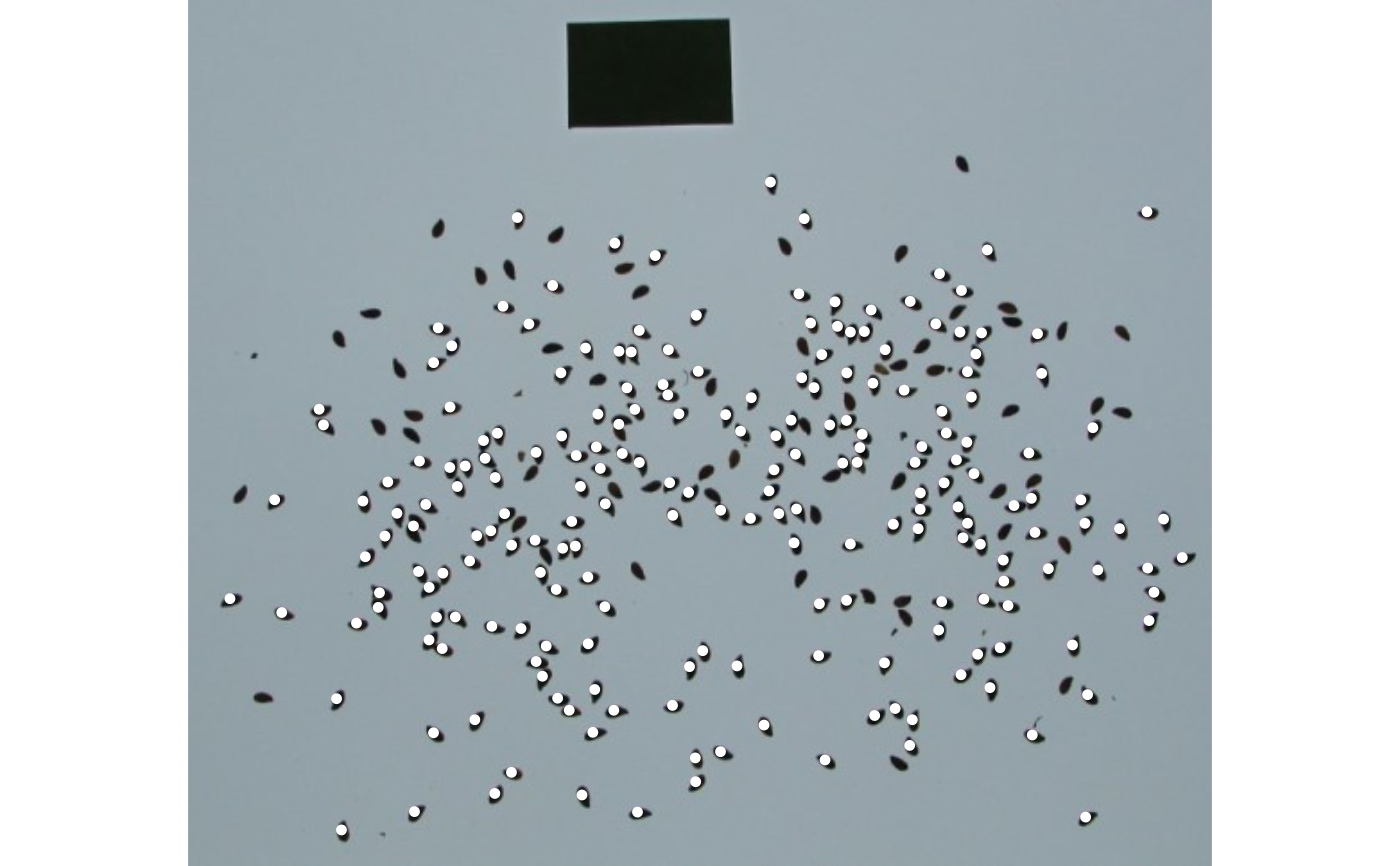
# Correct the measures based on the area of the largest object
# note that since the reference object
img <- image_pliman("flax_grains.jpg")
res <-
analyze_objects(img,
index = "GRAY",
marker = "point",
show_contour = FALSE,
reference = TRUE,
reference_area = 6,
reference_larger = TRUE,
lower_noise = 0.3)
top$results
#> id x y area area_ch perimeter radius_mean radius_min
#> 4 4 344.3132 104.74372 2436 2408.0 185.6102 27.45204 24.31796
#> 9 9 468.0383 55.44180 2311 2278.0 181.0244 26.77622 23.16169
#> 3 3 236.6572 338.80546 2310 2288.5 181.0244 26.69273 23.99117
#> 6 6 405.9755 76.41826 2297 2264.5 178.7817 26.58139 24.07681
#> 2 2 537.0532 400.81350 2289 2261.5 178.1960 26.55606 24.84882
#> radius_max radius_sd diam_mean diam_min diam_max major_axis minor_axis
#> 4 30.53131 1.7403323 54.90407 48.63592 61.06262 20.76326 18.04194
#> 9 31.04441 2.3392198 53.55243 46.32339 62.08881 20.69928 17.14476
#> 3 29.44025 1.2381808 53.38545 47.98234 58.88049 19.82571 17.91553
#> 6 30.02968 1.6596304 53.16279 48.15362 60.05937 19.82630 17.78272
#> 2 28.70321 0.9660995 53.11211 49.69764 57.40641 19.53438 18.01553
#> caliper length width radius_ratio theta eccentricity form_factor
#> 4 61.03278 61.02182 51.02160 1.255504 -0.9790241 0.4949248 0.8885535
#> 9 61.18823 61.07428 48.72944 1.340334 1.2628961 0.5603174 0.8862079
#> 3 57.69749 57.20139 51.99249 1.227128 -0.6370637 0.4282680 0.8858245
#> 6 59.48109 59.42578 50.82265 1.247245 1.1427598 0.4421814 0.9030764
#> 2 56.85948 56.53366 52.36854 1.155113 -0.8035065 0.3866007 0.9058576
#> narrow_factor asp_ratio rectangularity pd_ratio plw_ratio solidity convexity
#> 4 1.000180 1.196000 1.278091 3.041156 1.656592 1.011628 0.9187379
#> 9 1.001866 1.253334 1.287804 2.958484 1.648618 1.014486 0.8658923
#> 3 1.008673 1.100186 1.287464 3.137474 1.657825 1.009395 0.9111738
#> 6 1.000931 1.169277 1.314835 3.005691 1.621626 1.014352 0.8761289
#> 2 1.005763 1.079535 1.293397 3.133971 1.636293 1.012160 0.8794599
#> elongation circularity circularity_haralick circularity_norm coverage
#> 4 0.16387934 14.14250 15.77402 0.8584609 0.004556678
#> 9 0.20212827 14.17993 11.44664 0.8555300 0.004322858
#> 3 0.09106255 14.18607 21.55802 0.8551466 0.004320988
#> 6 0.14477098 13.91507 16.01645 0.8718206 0.004296670
#> 2 0.07367508 13.87235 27.48791 0.8745939 0.004281706
#' ########################### Example 1 #########################
# Correct the measures based on the area of the largest object
# note that since the reference object
img <- image_pliman("flax_grains.jpg")
res <-
analyze_objects(img,
index = "GRAY",
marker = "point",
show_contour = FALSE,
reference = TRUE,
reference_area = 6,
reference_larger = TRUE,
lower_noise = 0.3)
 # }
# \donttest{
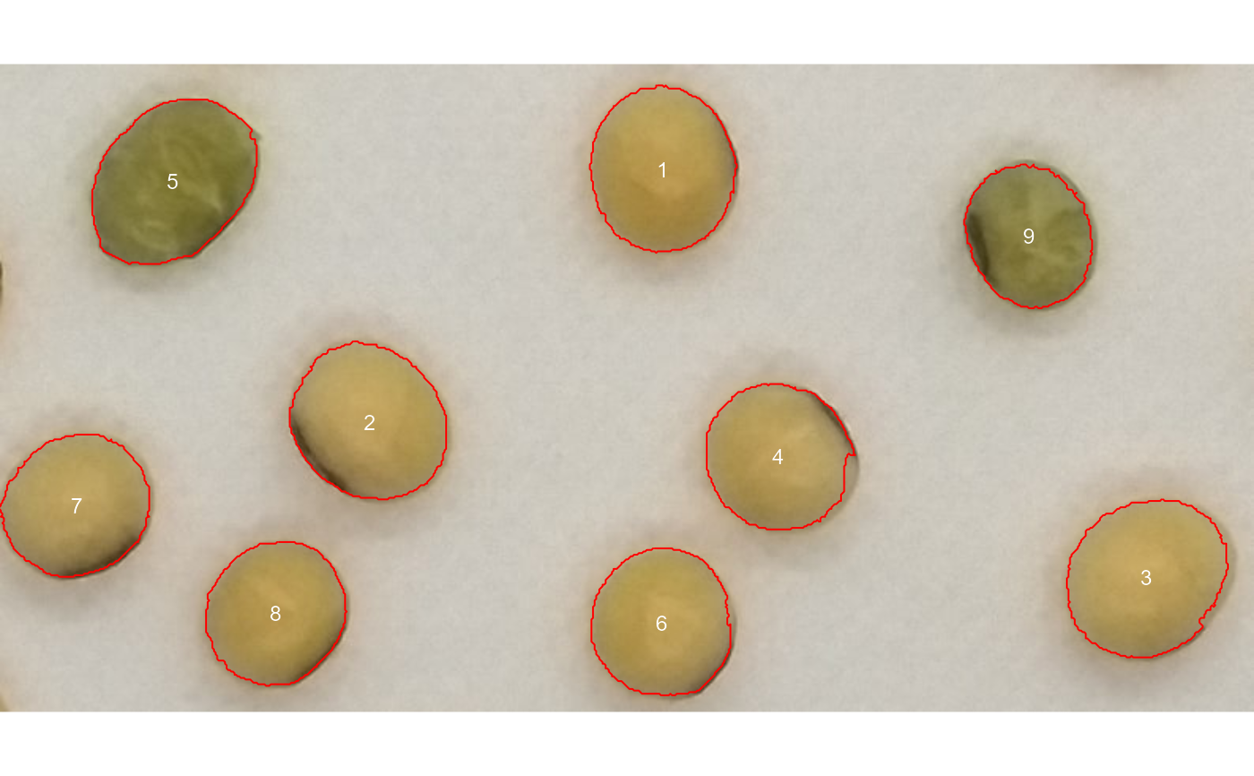
library(pliman)
img <- image_pliman("soy_green.jpg")
# Segment the foreground (grains) using the normalized blue index (NB, default)
# Shows the average value of the blue index in each object
rgb <-
analyze_objects(img,
marker = "id",
object_index = "B",
pixel_level_index = TRUE)
# }
# \donttest{
library(pliman)
img <- image_pliman("soy_green.jpg")
# Segment the foreground (grains) using the normalized blue index (NB, default)
# Shows the average value of the blue index in each object
rgb <-
analyze_objects(img,
marker = "id",
object_index = "B",
pixel_level_index = TRUE)
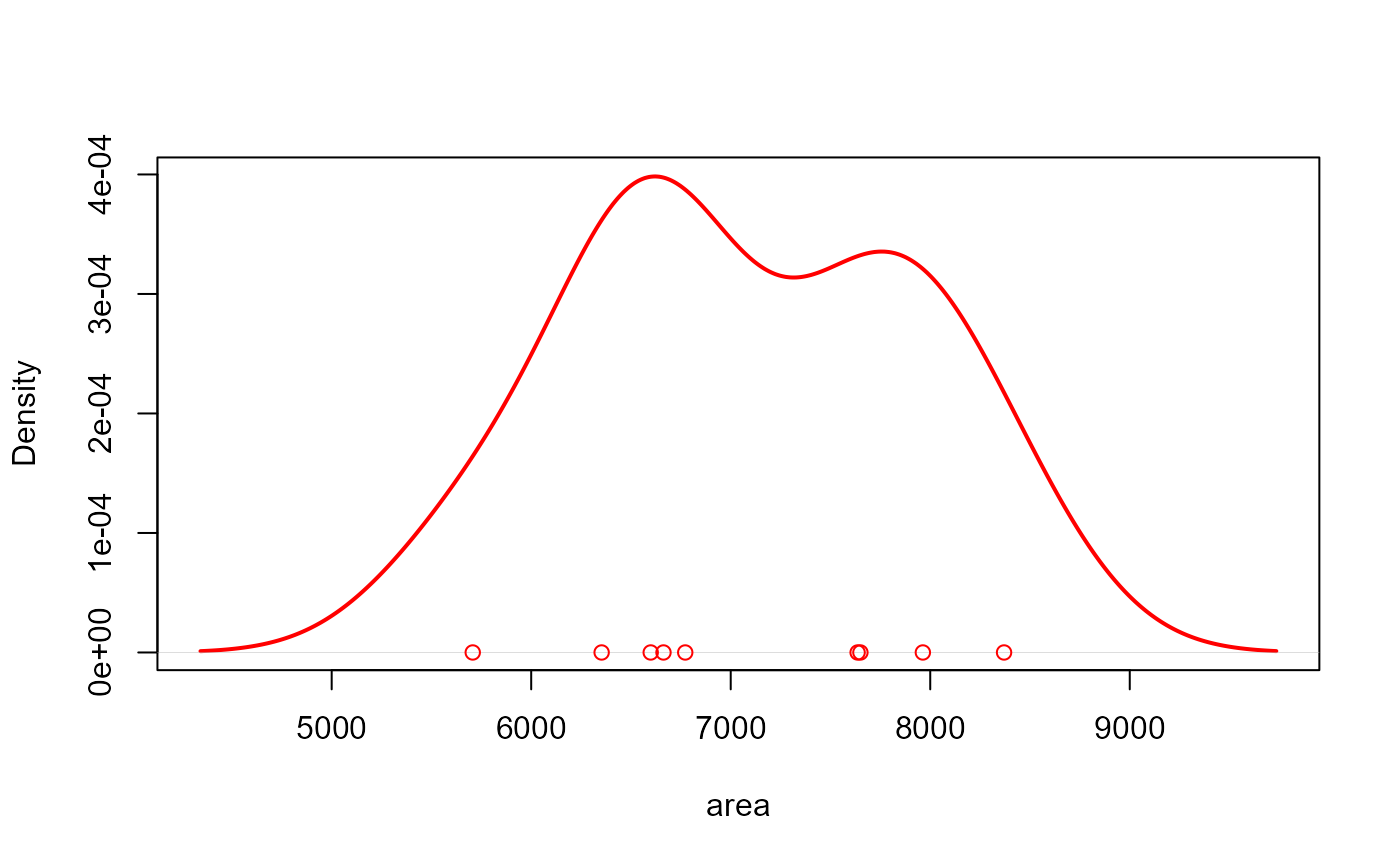
 # density of area
plot(rgb)
# density of area
plot(rgb)
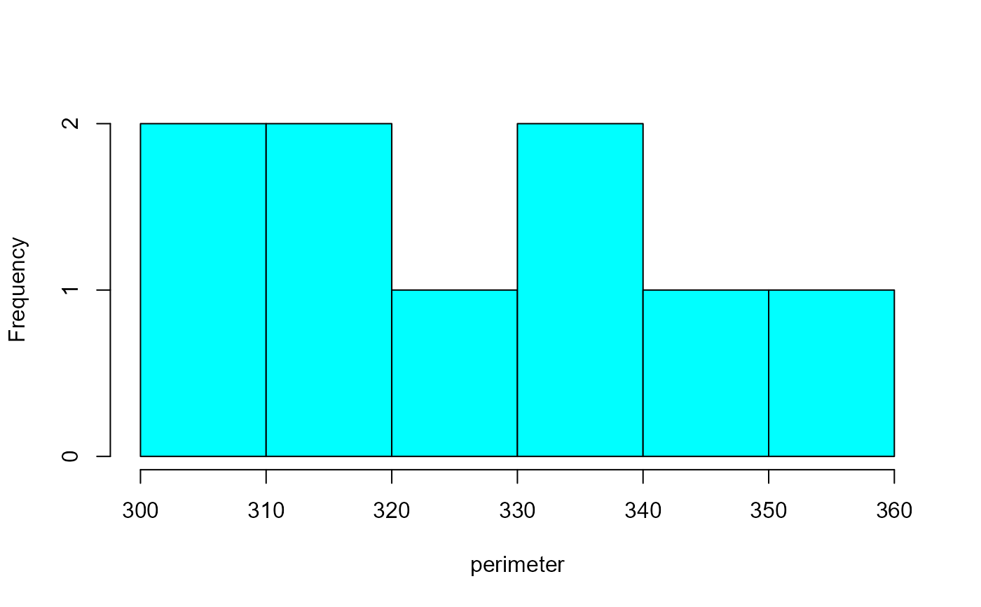
 # histogram of perimeter
plot(rgb, measure = "perimeter", type = "histogram") # or 'hist'
# histogram of perimeter
plot(rgb, measure = "perimeter", type = "histogram") # or 'hist'
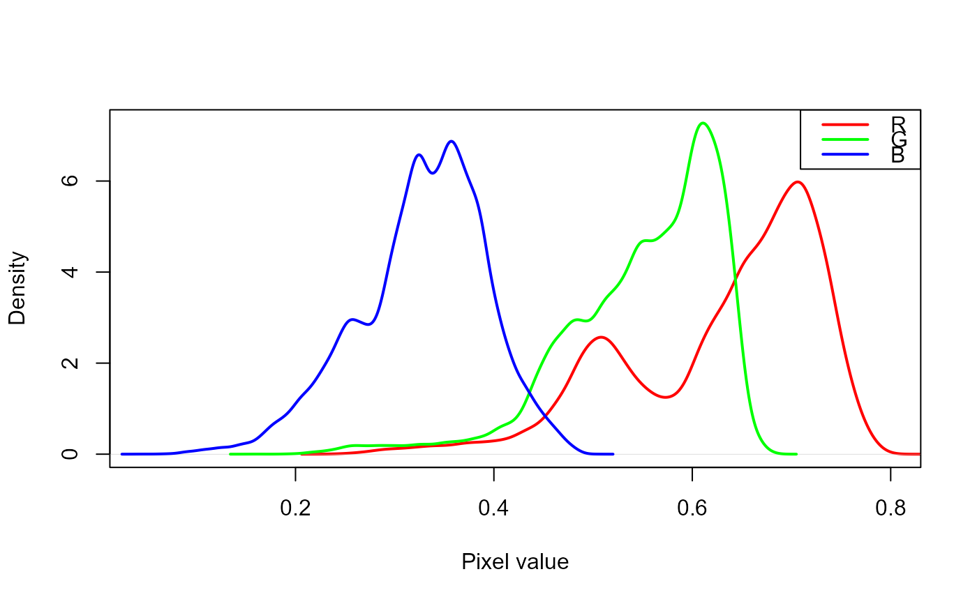
 # density of the blue (B) index
plot(rgb, which = "index")
# density of the blue (B) index
plot(rgb, which = "index")
 # }
# }