Analyzing objects in an image
Tiago Olivoto
2023-10-22
Source:vignettes/analyze_objects.Rmd
analyze_objects.RmdGetting started
The function analyze_objects() can be used to count
objects in an image. Let us start with a simple example with the image
object_300dpi.png available on the GitHub
page. To facilitate the image importation from this folder, a helper
function image_pliman() is used.
library(pliman)
#> |==========================================================|
#> | Tools for Plant Image Analysis (pliman 2.1.0)            |
#> | Author: Tiago Olivoto                                    |
#> | Type `citation('pliman')` to know how to cite pliman     |
#> | Visit 'http://bit.ly/pkg_pliman' for a complete tutorial |
#> |==========================================================|
img <- image_pliman("objects_300dpi.jpg", plot = TRUE)
The above image was produced with Microsoft PowerPoint. It has a known resolution of 300 dpi (dots per inch) and shows four objects
- Larger square: 10 x 10 cm (100 cm2)
- Smaller square: 5 x 5 cm (25 cm2)
- Rectangle: 4 x 2 cm (8 cm2)
- Circle: 3 cm in diameter (~7.08 cm2)
To count the objects in the image we use
analyze_objects() and inform the image object (the only
mandatory argument). First, we use image_binary() to see
the most suitable index to segment the objects from the background. By
default, the R, G, B (first row) and their normalized values (second
row) are used.
image_binary(img)
Analyzing objects
img_res <-
  analyze_objects(img,
                  marker = "id",
                  index = "B") # use blue index to segment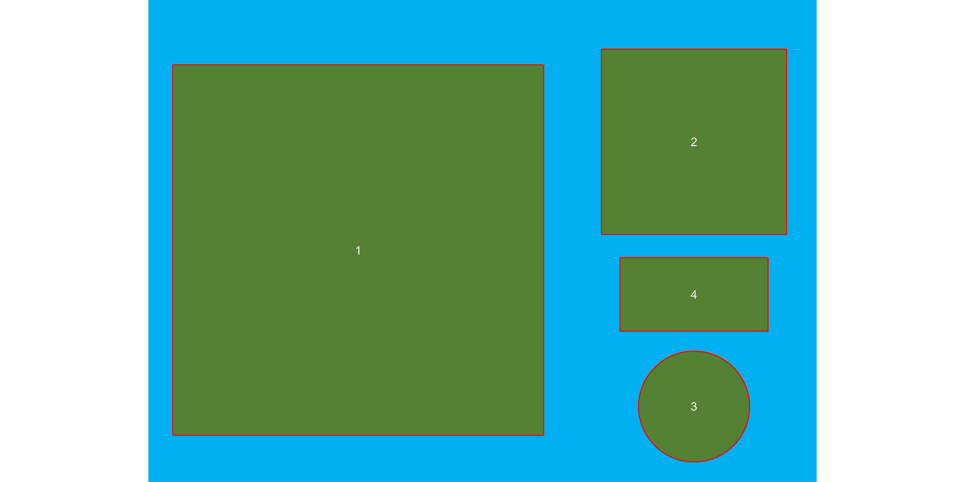
Adjusting object measures
The results were stored in img_res. Since there is no
scale declared in the above example, we have no idea about the actual
area of the objects in cm2, only in pixels. In this case, we
use get_measures() to adjust the measures from pixels to
metric units.
There are two main ways of adjusting the object measures (from pixels to cm, for example). The first one is to declare the known area, perimeter, or radius of a given object. The measure for the other objects will be then computed by a simple rule of three. The second one is by declaring a known image resolution in dpi (dots per inch). In this case, the perimeter, area, and radius will be adjusted by the informed dpi.
Declaring a known value
Since we have known the area of the larger square (object 1), let us adjust the area of the other objects in the image using that.
get_measures(img_res,
             id = 1,
             area ~ 100) |>
  str()
#> -----------------------------------------
#> measures corrected with:
#> object id: 1
#> area     : 100
#> -----------------------------------------
#> Total    : 40.001
#> Average  : 13.334
#> -----------------------------------------
#> Classes 'measures' and 'data.frame': 3 obs. of  34 variables:
#>  $ id                  : num  2 3 4
#>  $ x                   : num  1737 1737 1736
#>  $ y                   : num  452 1295 938
#>  $ area                : num  25 7.05 7.95
#>  $ area_ch             : num  24.92 7.05 7.9
#>  $ perimeter           : num  19.9 10.1 11.9
#>  $ radius_mean         : num  2.86 1.49 1.67
#>  $ radius_min          : num  2.492 1.482 0.988
#>  $ radius_max          : num  3.53 1.51 2.23
#>  $ radius_sd           : num  0.31434 0.00396 0.42388
#>  $ diam_mean           : num  5.73 2.99 3.34
#>  $ diam_min            : num  4.98 2.96 1.98
#>  $ diam_max            : num  7.06 3.02 4.45
#>  $ major_axis          : num  2.04 1.06 1.48
#>  $ minor_axis          : num  2.036 1.053 0.874
#>  $ caliper             : num  7.01 3 4.43
#>  $ length              : num  5 3 3.99
#>  $ width               : num  4.99 3 1.98
#>  $ radius_ratio        : num  1.42 1.02 2.25
#>  $ theta               : num  -1.57 0.459 0
#>  $ eccentricity        : num  0.0505 0.1114 0.808
#>  $ form_factor         : num  0.79 0.873 0.704
#>  $ narrow_factor       : num  1.4 1 1.11
#>  $ asp_ratio           : num  1 1 2.01
#>  $ rectangularity      : num  0.998 1.278 0.994
#>  $ pd_ratio            : num  2.85 3.36 2.69
#>  $ plw_ratio           : num  2 1.68 2
#>  $ solidity            : num  1 1 1.01
#>  $ convexity           : num  0.75 0.909 0.836
#>  $ elongation          : num  0.00169 0.00113 0.50318
#>  $ circularity         : num  15.9 14.4 17.8
#>  $ circularity_haralick: num  9.11 377.4 3.94
#>  $ circularity_norm    : num  0.787 0.868 0.7
#>  $ coverage            : num  0.1068 0.0301 0.034
The same can be used to adjust the measures based on the perimeter or radius. Let us adjust the perimeter of objects by the perimeter of object 2 (20 cm).
get_measures(img_res,
             id = 2,
             perimeter ~ 20) |>
  str()
#> -----------------------------------------
#> measures corrected with:
#> object id: 2
#> perimeter     : 20
#> -----------------------------------------
#> Total    : 62.081
#> Average  : 20.694
#> -----------------------------------------
#> Classes 'measures' and 'data.frame': 3 obs. of  34 variables:
#>  $ id                  : num  1 3 4
#>  $ x                   : num  668 1737 1736
#>  $ y                   : num  797 1295 938
#>  $ area                : num  100.52 7.09 7.99
#>  $ area_ch             : num  100.35 7.09 7.94
#>  $ perimeter           : num  40 10.1 11.9
#>  $ radius_mean         : num  5.75 1.5 1.67
#>  $ radius_min          : num  5.01 1.49 0.99
#>  $ radius_max          : num  7.08 1.51 2.23
#>  $ radius_sd           : num  0.63056 0.00397 0.42499
#>  $ diam_mean           : num  11.5 3 3.35
#>  $ diam_min            : num  10.02 2.97 1.98
#>  $ diam_max            : num  14.16 3.03 4.46
#>  $ major_axis          : num  4.09 1.06 1.49
#>  $ minor_axis          : num  4.088 1.056 0.876
#>  $ caliper             : num  14.08 3.01 4.45
#>  $ length              : num  14.16 3.01 4
#>  $ width               : num  14.15 3.01 1.99
#>  $ radius_ratio        : num  1.41 1.02 2.25
#>  $ theta               : num  0.783 0.459 0
#>  $ eccentricity        : num  0.0253 0.1114 0.808
#>  $ form_factor         : num  0.788 0.873 0.704
#>  $ narrow_factor       : num  0.995 1 1.112
#>  $ asp_ratio           : num  1 1 2.01
#>  $ rectangularity      : num  1.992 1.278 0.994
#>  $ pd_ratio            : num  2.84 3.36 2.69
#>  $ plw_ratio           : num  1.41 1.68 2
#>  $ solidity            : num  1 1 1.01
#>  $ convexity           : num  0.75 0.909 0.836
#>  $ elongation          : num  0.00043 0.00113 0.50318
#>  $ circularity         : num  15.9 14.4 17.8
#>  $ circularity_haralick: num  9.12 377.4 3.94
#>  $ circularity_norm    : num  0.787 0.868 0.7
#>  $ coverage            : num  0.4274 0.0301 0.034
Declaring the image resolution
If the image resolution is known, all the measures will be adjusted
according to this resolution. Let us to see a numerical example with
pixels_to_cm(). This function converts the number of pixels
(\(px\)) to cm, considering the image
resolution in \(dpi\), as follows:
\(cm = px \times (2.54/dpi)\). Since we
know the number of pixels of the larger square, its perimeter in cm is
given by
# number of pixels for the highest square perimeter
ls_px <- img_res$results$perimeter[1]
pixels_to_cm(px = ls_px, dpi = 300)
#> [1] 39.9294
The perimeter of object 1 adjusted by the image resolution is very
close to the true (40 cm). Bellow, the values of all measures are
adjusted by declaring the dpi argument in
get_measures().
get_measures(img_res, dpi = 300) |> str()
#> Classes 'measures' and 'data.frame': 4 obs. of  34 variables:
#>  $ id                  : num  1 2 3 4
#>  $ x                   : num  668 1737 1737 1736
#>  $ y                   : num  797 452 1295 938
#>  $ area                : num  99.98 25 7.05 7.95
#>  $ area_ch             : num  99.81 24.91 7.05 7.9
#>  $ perimeter           : num  39.9 19.9 10.1 11.9
#>  $ radius_mean         : num  5.73 2.86 1.49 1.67
#>  $ radius_min          : num  4.994 2.491 1.482 0.988
#>  $ radius_max          : num  7.06 3.53 1.51 2.23
#>  $ radius_sd           : num  0.62885 0.31432 0.00396 0.42384
#>  $ diam_mean           : num  11.46 5.73 2.99 3.34
#>  $ diam_min            : num  9.99 4.98 2.96 1.98
#>  $ diam_max            : num  14.12 7.06 3.02 4.45
#>  $ major_axis          : num  4.08 2.04 1.06 1.48
#>  $ minor_axis          : num  4.077 2.036 1.053 0.874
#>  $ caliper             : num  14.05 7.01 3 4.43
#>  $ length              : num  14.12 5 3 3.99
#>  $ width               : num  14.11 4.99 3 1.98
#>  $ radius_ratio        : num  1.41 1.42 1.02 2.25
#>  $ theta               : num  0.783 -1.57 0.459 0
#>  $ eccentricity        : num  0.0253 0.0505 0.1114 0.808
#>  $ form_factor         : num  0.788 0.79 0.873 0.704
#>  $ narrow_factor       : num  0.995 1.402 1 1.112
#>  $ asp_ratio           : num  1 1 1 2.01
#>  $ rectangularity      : num  1.992 0.998 1.278 0.994
#>  $ pd_ratio            : num  2.84 2.85 3.36 2.69
#>  $ plw_ratio           : num  1.41 2 1.68 2
#>  $ solidity            : num  1 1 1 1.01
#>  $ convexity           : num  0.75 0.75 0.909 0.836
#>  $ elongation          : num  0.00043 0.00169 0.00113 0.50318
#>  $ circularity         : num  15.9 15.9 14.4 17.8
#>  $ circularity_haralick: num  9.12 9.11 377.4 3.94
#>  $ circularity_norm    : num  0.787 0.787 0.868 0.7
#>  $ coverage            : num  0.4274 0.1068 0.0301 0.034
Counting crop grains
Here, we will count the grains in the image
soybean_touch.jpg. This image has a cyan background and
contains 30 soybean grains that touch with each other. Two segmentation
strategies are used. The first one is by using is image segmentation
based on color indexes.
soy <-        image_pliman("soybean_touch.jpg")
grain <-      image_pliman("soybean_grain.jpg")
background <- image_pliman("la_back.jpg")
image_combine(soy, grain, background, ncol = 3)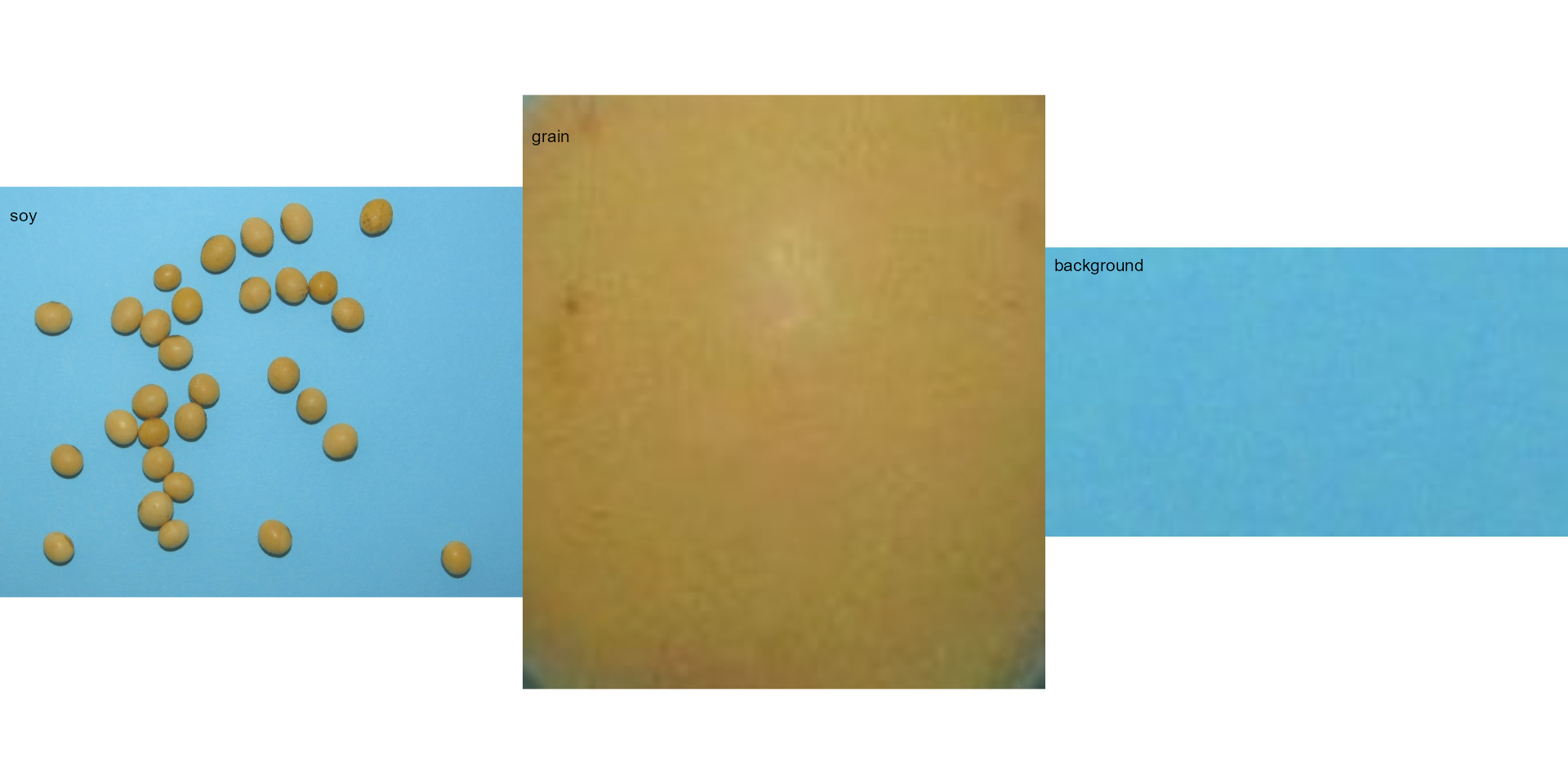
The function analyze_objects() segment the image using
as default the normalized blue index, as follows \(NB = (B/(R+G+B))\), where \(R\), \(G\), and \(B\) are the red, green, and blue bands.
Objects are count and the segmented objects are colored with random
permutations.
count2 <-
  analyze_objects(soy,
                  index = "NB") # default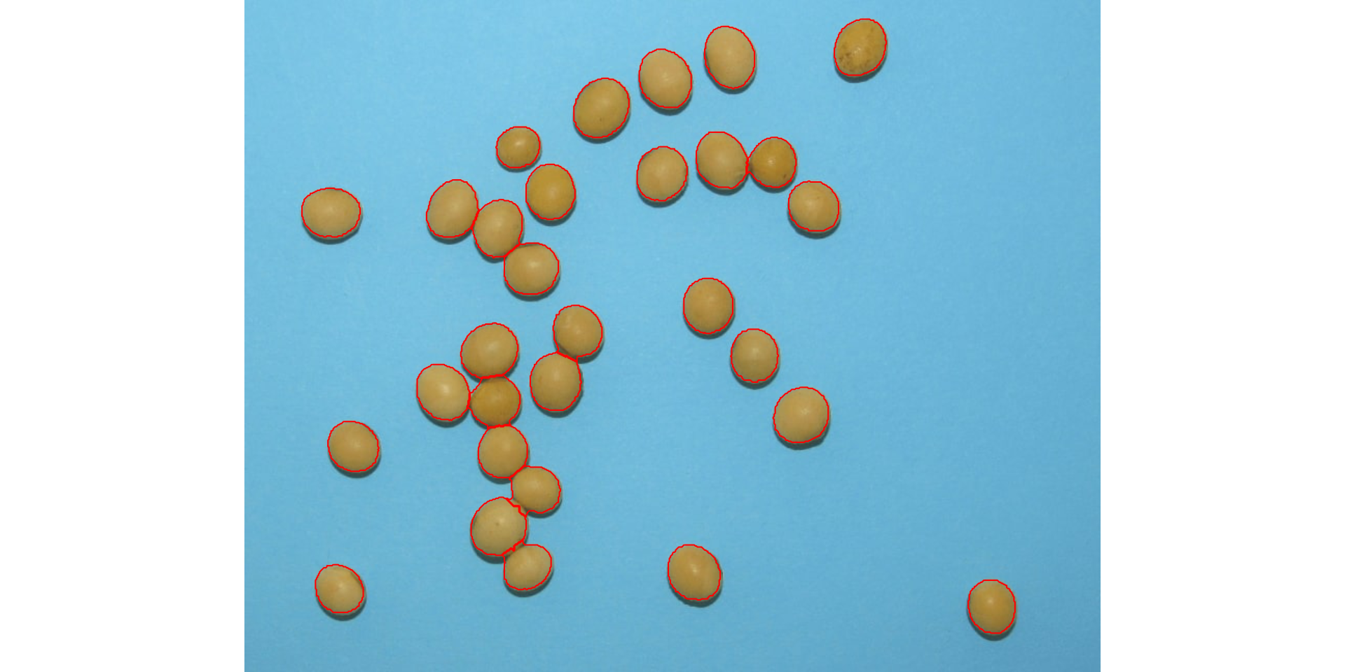
Users can set show_contour = FALSE to remove the contour
line and identify the objects (in this example the grains) by using the
arguments marker = "id". The color of the background can
also be changed with col_background.
count <-
  analyze_objects(soy,
                  show_contour = FALSE,
                  marker = "id",
                  show_segmentation = FALSE,
                  col_background = "white",
                  index = "NB") # default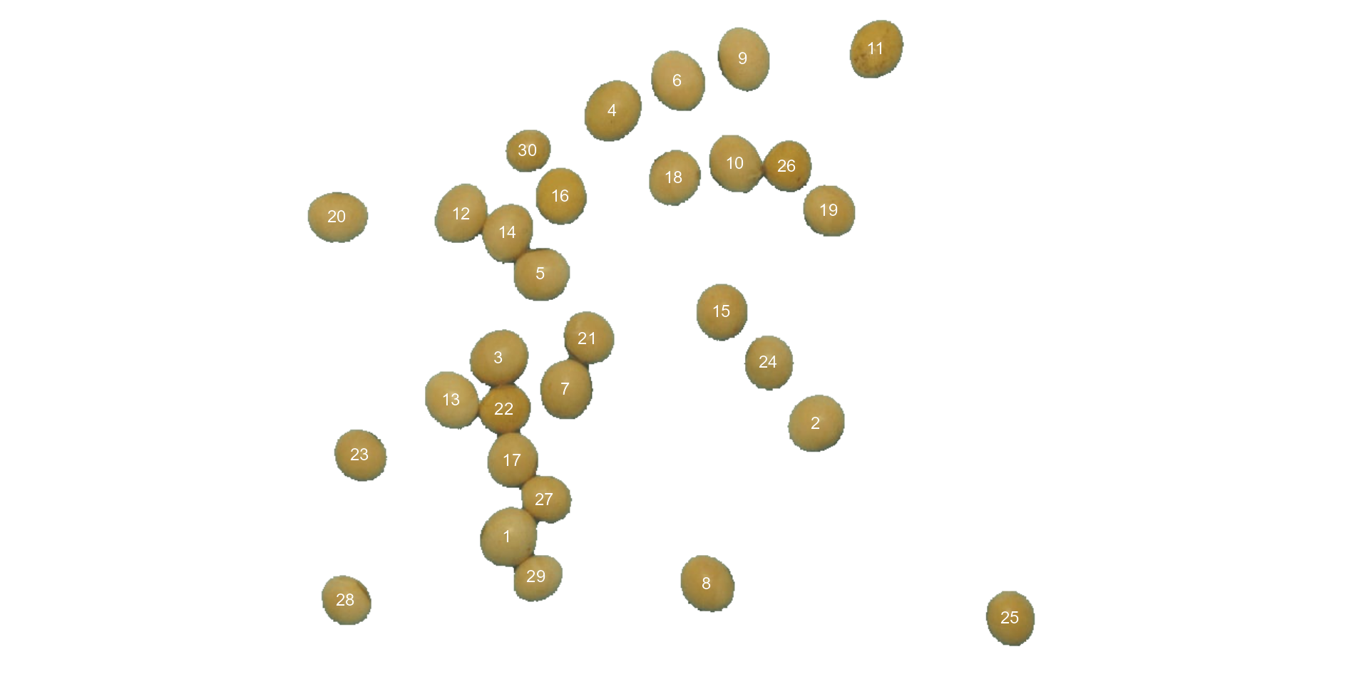
# Get the object measures
measures <- get_measures(count)
str(measures)
#> Classes 'measures' and 'data.frame': 30 obs. of  34 variables:
#>  $ id                  : num  1 2 3 4 5 6 7 8 9 10 ...
#>  $ x                   : num  245 537 237 344 277 ...
#>  $ y                   : num  509 401 339 105 260 ...
#>  $ area                : num  2279 2289 2310 2436 2159 ...
#>  $ area_ch             : num  2304 2262 2288 2408 2122 ...
#>  $ perimeter           : num  184 178 181 186 172 ...
#>  $ radius_mean         : num  26.5 26.6 26.7 27.5 25.8 ...
#>  $ radius_min          : num  23 24.8 24 24.3 24.2 ...
#>  $ radius_max          : num  29.4 28.7 29.4 30.5 28 ...
#>  $ radius_sd           : num  1.375 0.966 1.238 1.74 0.801 ...
#>  $ diam_mean           : num  53 53.1 53.4 54.9 51.5 ...
#>  $ diam_min            : num  45.9 49.7 48 48.6 48.5 ...
#>  $ diam_max            : num  58.8 57.4 58.9 61.1 56.1 ...
#>  $ major_axis          : num  19.3 19.5 19.8 20.8 18.7 ...
#>  $ minor_axis          : num  18.2 18 17.9 18 17.7 ...
#>  $ caliper             : num  57.3 56.9 57.7 61 54.4 ...
#>  $ length              : num  56.6 56.5 57.2 61 54 ...
#>  $ width               : num  51.5 52.4 52 51 50.5 ...
#>  $ radius_ratio        : num  1.28 1.16 1.23 1.26 1.16 ...
#>  $ theta               : num  -0.828 -0.804 -0.637 -0.979 -0.217 ...
#>  $ eccentricity        : num  0.328 0.387 0.428 0.495 0.325 ...
#>  $ form_factor         : num  0.85 0.906 0.886 0.889 0.92 ...
#>  $ narrow_factor       : num  1.01 1.01 1.01 1 1.01 ...
#>  $ asp_ratio           : num  1.1 1.08 1.1 1.2 1.07 ...
#>  $ rectangularity      : num  1.28 1.29 1.29 1.28 1.26 ...
#>  $ pd_ratio            : num  3.2 3.13 3.14 3.04 3.16 ...
#>  $ plw_ratio           : num  1.7 1.64 1.66 1.66 1.64 ...
#>  $ solidity            : num  0.989 1.012 1.009 1.012 1.017 ...
#>  $ convexity           : num  0.887 0.879 0.911 0.919 0.898 ...
#>  $ elongation          : num  0.089 0.0737 0.0911 0.1639 0.0643 ...
#>  $ circularity         : num  14.8 13.9 14.2 14.1 13.7 ...
#>  $ circularity_haralick: num  19.3 27.5 21.6 15.8 32.2 ...
#>  $ circularity_norm    : num  0.821 0.875 0.855 0.858 0.887 ...
#>  $ coverage            : num  0.00426 0.00428 0.00432 0.00456 0.00404 0.0043 0.00414 0.00406 0.00432 0.00405 ...
In the following example, we will select objects with an area above
the average of all objects by using lower_size = 2057.36.
Additionally, we will use the argument
show_original = FALSE to show the results as colors
(non-original image).
analyze_objects(soy,
                marker = "id",
                show_original = FALSE,
                lower_size = 2057.36,
                index = "NB") # default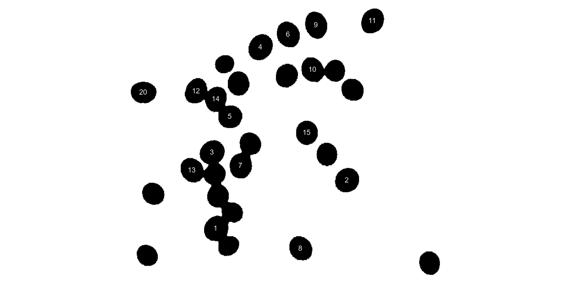
Users can also use the topn_* arguments to select the
top n objects based on either smaller or largest areas.
Let’s see how to point out the 5 grains with the smallest area, showing
the original grains in a blue background. We will also use the argument
index to choose a personalized index to segment the image.
Just for comparison, we will set up explicitly the normalized blue index
by calling index = "B/(R+G+B)".
analyze_objects(soy,
                marker = "id",
                topn_lower = 5,
                col_background = "blue",
                index = "B/(R+G+B)") # default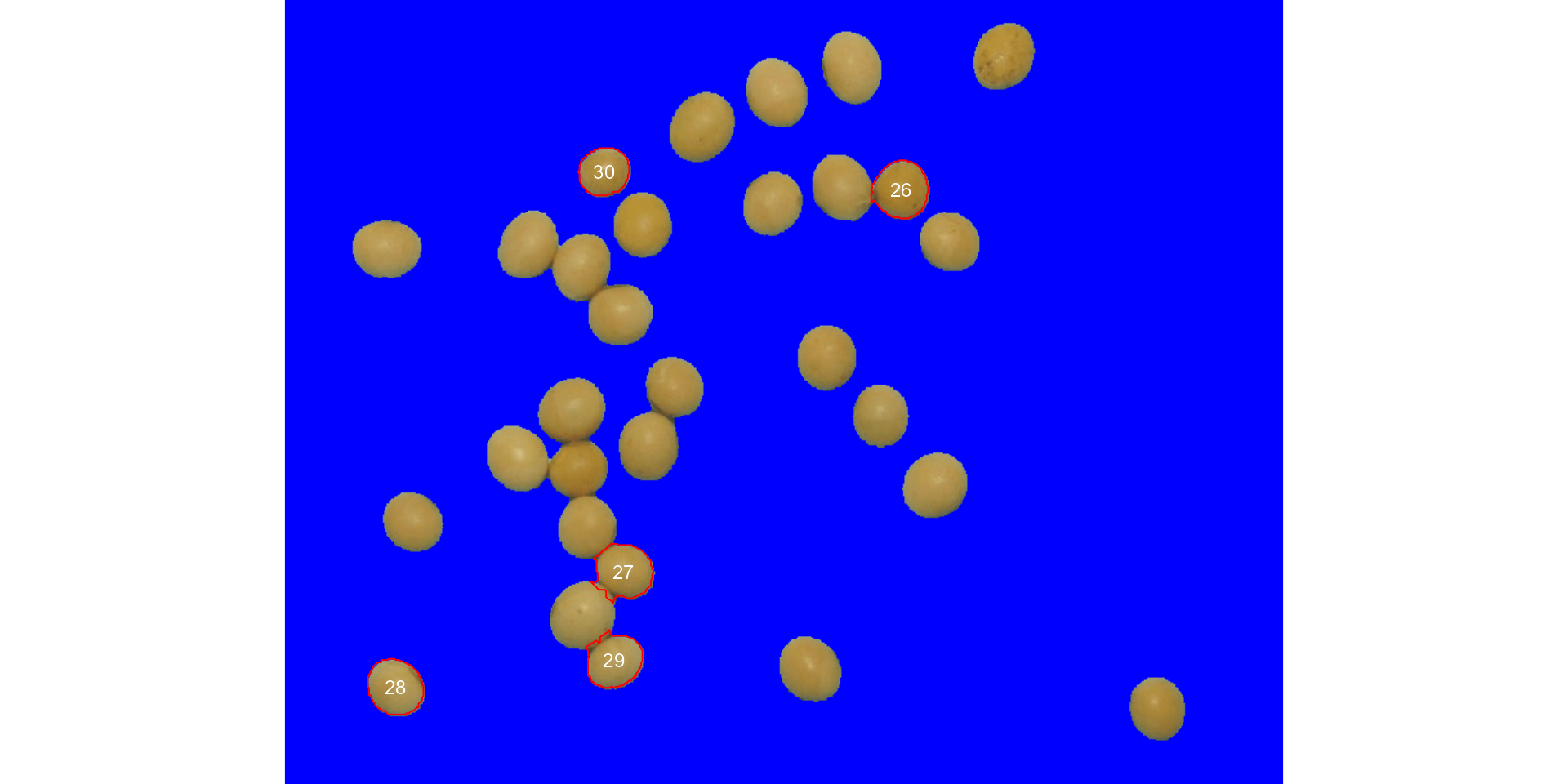
Using sample palettes
Sometimes it is difficult to choose an image index that segments the
image efficiently (even using index ). In
pliman users have an alternative image segmentation
strategy that is using sample color palettes. In this case, users can
say to analyze_objects which color palettes are to be used
for background and foreground. A generalized linear model (binomial
family) is then used to predict the value of each pixel (background or
foreground). Let’s see how the grains of the above image can be counted
with this strategy.
analyze_objects(img = soy,
                background = background,
                foreground = grain)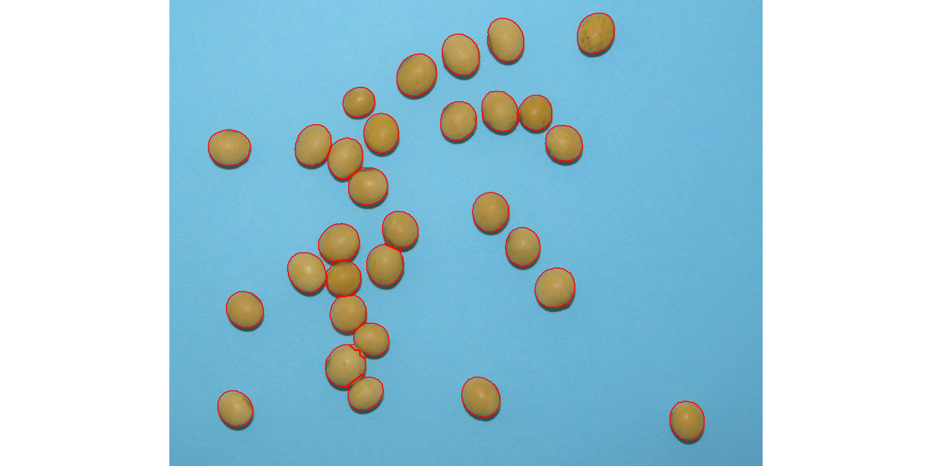
Provided that the images are stored in the current working directory (or subdirectory), users can count the objects with no need to first import the image into the R environment. In this case, image names need to be declared as characters. Assuming that soy, background, and grain are the images saved into the current working directory, the same result as above is obtained with
analyze_objects(img = "soy",
                background = "background",
                foreground = "grain")
Leaf shape
The function analyze_objects() computes a range of
object features that can be used to study leaf shape. As a motivating
example, I will use the image potato_leaves.png, which was
gathered from Gupta et al. (2020)1
potato <- image_pliman("potato_leaves.jpg", plot = TRUE)
pot_meas <-
  analyze_objects(potato,
                  watershed = FALSE,
                  marker = "id",
                  show_chull = TRUE) # shows the convex hull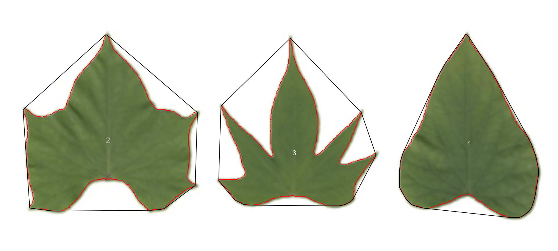
str(pot_meas)
#> List of 16
#>  $ results         :'data.frame':    3 obs. of  34 variables:
#>   ..$ id                  : num [1:3] 1 2 3
#>   ..$ x                   : num [1:3] 639 147 401
#>   ..$ y                   : num [1:3] 167 162 180
#>   ..$ area                : num [1:3] 28715 32982 19565
#>   ..$ area_ch             : num [1:3] 30490 42835 34718
#>   ..$ perimeter           : num [1:3] 754 935 1132
#>   ..$ radius_mean         : num [1:3] 98.1 105 81.8
#>   ..$ radius_min          : num [1:3] 68.5 52.7 27.9
#>   ..$ radius_max          : num [1:3] 147 143 140
#>   ..$ radius_sd           : num [1:3] 19.6 21.3 26.3
#>   ..$ diam_mean           : num [1:3] 196 210 164
#>   ..$ diam_min            : num [1:3] 137.1 105.5 55.9
#>   ..$ diam_max            : num [1:3] 295 287 279
#>   ..$ major_axis          : num [1:3] 78.5 80 62.2
#>   ..$ minor_axis          : num [1:3] 62 71.3 59.2
#>   ..$ caliper             : num [1:3] 258 257 233
#>   ..$ length              : num [1:3] 258 244 219
#>   ..$ width               : num [1:3] 191 246 228
#>   ..$ radius_ratio        : num [1:3] 2.15 2.72 5
#>   ..$ theta               : num [1:3] 1.428 -0.136 0.536
#>   ..$ eccentricity        : num [1:3] 0.614 0.453 0.307
#>   ..$ form_factor         : num [1:3] 0.635 0.474 0.192
#>   ..$ narrow_factor       : num [1:3] 1 1.06 1.06
#>   ..$ asp_ratio           : num [1:3] 1.352 0.991 0.961
#>   ..$ rectangularity      : num [1:3] 1.71 1.82 2.55
#>   ..$ pd_ratio            : num [1:3] 2.92 3.63 4.86
#>   ..$ plw_ratio           : num [1:3] 1.68 1.91 2.53
#>   ..$ solidity            : num [1:3] 0.942 0.77 0.564
#>   ..$ convexity           : num [1:3] 0.915 0.736 0.563
#>   ..$ elongation          : num [1:3] 0.26027 -0.00948 -0.04045
#>   ..$ circularity         : num [1:3] 19.8 26.5 65.5
#>   ..$ circularity_haralick: num [1:3] 5.02 4.93 3.1
#>   ..$ circularity_norm    : num [1:3] 0.628 0.468 0.187
#>   ..$ coverage            : num [1:3] 0.1332 0.153 0.0908
#>  $ statistics      :'data.frame':    7 obs. of  2 variables:
#>   ..$ stat : chr [1:7] "n" "min_area" "mean_area" "max_area" ...
#>   ..$ value: num [1:7] 3 19565 27087 32982 6855 ...
#>  $ object_rgb      : NULL
#>  $ object_index    : NULL
#>  $ efourier        : NULL
#>  $ efourier_norm   : NULL
#>  $ efourier_error  : NULL
#>  $ efourier_power  : NULL
#>  $ efourier_minharm: NULL
#>  $ veins           : NULL
#>  $ angles          : NULL
#>  $ width_at        : NULL
#>  $ mask            : NULL
#>  $ pcv             : NULL
#>  $ contours        :List of 3
#>   ..$ 1: int [1:641, 1:2] 634 634 633 633 632 631 631 630 630 629 ...
#>   ..$ 2: int [1:806, 1:2] 144 144 144 143 143 142 142 142 141 141 ...
#>   ..$ 3: int [1:982, 1:2] 395 395 395 394 394 394 394 394 394 394 ...
#>  $ parms           :List of 1
#>   ..$ index: chr "NB"
#>  - attr(*, "class")= chr "anal_obj"
Three key measures (in pixel units) are:
-
areathe area of the object. -
area_chthe area of the convex hull. -
perimeterthe perimeter of the object.
Using these measures, circularity and solidity are computed as shown in (Gupta et al, 2020).
\[ circularity = 4\pi(area / perimeter^2)\]
\[solidity = area / area\_ch\]
Circularity is influenced by serrations and lobing. Solidity is sensitive to leaves with deep lobes, or with a distinct petiole, and can be used to distinguish leaves lacking such structures. Unlike circularity, it is not very sensitive to serrations and minor lobings, since the convex hull remains largely unaffected.
Object contour
Users can also obtain the object contour and convex hull as follows:
cont <-
  object_contour(potato,
                 watershed = FALSE,
                 plot = FALSE)
plot(potato)
plot_contour(cont, col = "red", lwd = 3)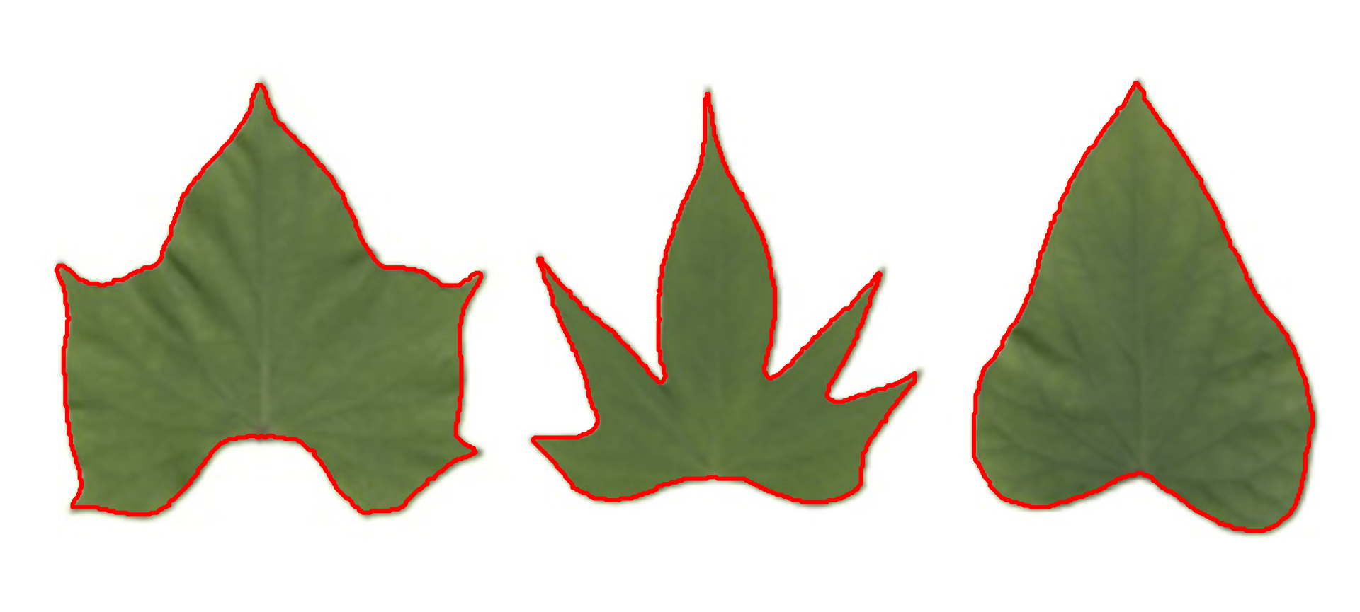
Convex hull
The function object_contour() returns a list with the
coordinate points for each object contour that can be further used to
obtain the convex hull with conv_hull().
conv <- conv_hull(cont)
plot(potato)
plot_contour(conv, col = "red", lwd = 3)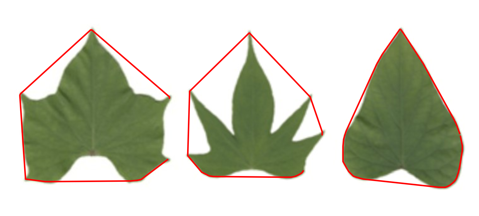
Area of the convex hull
Then, the area of the convex hull can be obtained with
poly_area().
(area <- poly_area(conv))
#> [1] 30490 42835 34718
Leaves as base plot
# create a data frame for contour and convex hull
df_cont <-
  do.call(rbind,
          lapply(seq_along(cont), function(i){
            transform(as.data.frame(cont[[i]]), object = names(cont[i]))
          }))

df_conv <-
  do.call(rbind,
          lapply(seq_along(conv), function(i){
            transform(as.data.frame(conv[[i]]), object = names(conv[i]))
          }))


# plot the objects
palette(c("red","blue","green"))
with(df_cont,
     plot(V1, V2,
          cex = 0.5,
          col = object,
          xlab = NA,
          ylab = NA,
          axes = F))
with(subset(df_conv, object == 1),
     polygon(V1, V2,
             col = rgb(1, 0, 0, 0.2),
             border = NA))
with(subset(df_conv, object == 2),
     polygon(V1, V2,
             col = rgb(0, 0, 1, 0.2),
             border = NA))
with(subset(df_conv, object == 3),
     polygon(V1, V2,
             col = rgb(0, 1, 0, 0.2),
             border = NA))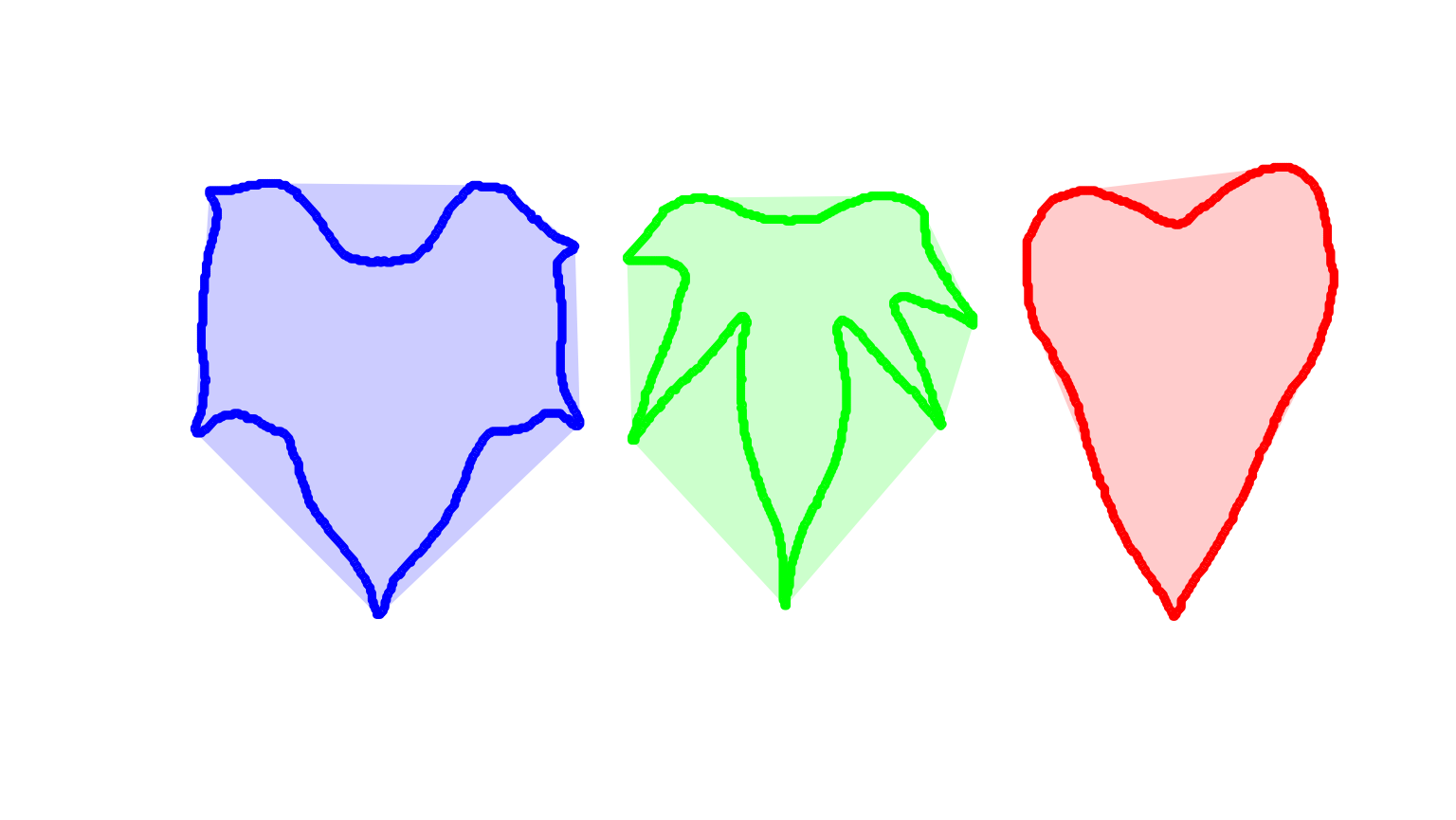
Or do the same with ggplot2
library(ggplot2)
ggplot(df_cont, aes(V1, V2, group = object)) +
  geom_polygon(aes(fill = object)) +
  geom_polygon(data = df_conv,
               aes(V1, V2, fill = object),
               alpha = 0.3) +
  theme_void() +
  theme(legend.position = "bottom")
Batch processing
In plant image analysis, frequently it is necessary to process more
than one image. For example, in plant breeding, the number of grains per
plant (e.g., wheat) is frequently used in the indirect selection of
high-yielding plants. In pliman, batch processing can be
done when the user declares the argument pattern.
The following example would be used to count the objects in the
images with a pattern name "trat" (e.g.,
"trat1", "trat2", "tratn") saved
into the subfolder “originals" in the current working
directory. The processed images will be saved into the subfolder
"processed". The object list_res will be a
list with two objects (results and statistics)
for each image.
To speed up the processing time, especially for a large number of
images, the argument parallel = TRUE can be used. In this
case, the images are processed asynchronously (in parallel) in separate
R sessions running in the background on the same machine.
The number of sections is set up to 50% of available cores. This number
can be controlled explicitly with the argument workers.
list_res <-
  analyze_objects(pattern = "trat", # matches the name pattern in 'originals' subfolder
                  dir_original = "originals",
                  dir_processed = "processed",
                  parallel = TRUE, # parallel processing
                  workers = 8, # 8 multiple sections
                  save_image = TRUE)