![[Stable]](figures/lifecycle-stable.svg)
Computes the multi-trait genotype-ideotype distance index, MGIDI, (Olivoto and Nardino, 2020), used to select genotypes in plant breeding programs based on multiple traits.The MGIDI index is computed as follows: \[MGIDI_i = \sqrt{\sum\limits_{j = 1}^f(F_{ij} - {F_j})^2}\]
where \(MGIDI_i\) is the multi-trait genotype-ideotype distance index for the ith genotype; \(F_{ij}\) is the score of the ith genotype in the jth factor (i = 1, 2, ..., g; j = 1, 2, ..., f), being g and f the number of genotypes and factors, respectively, and \(F_j\) is the jth score of the ideotype. The genotype with the lowest MGIDI is then closer to the ideotype and therefore should presents desired values for all the analyzed traits.
Usage
mgidi(
  .data,
  use_data = "blup",
  SI = 15,
  mineval = 1,
  ideotype = NULL,
  weights = NULL,
  use = "complete.obs",
  verbose = TRUE
)
Arguments
- .data
An object fitted with the function
gafem(),gamem()or a two-way table with BLUPs for genotypes in each trait (genotypes in rows and traits in columns). In the last case, row names must contain the genotypes names.- use_data
Define which data to use if
.datais an object of classgamem. Defaults to"blup"(the BLUPs for genotypes). Use"pheno"to use phenotypic means instead BLUPs for computing the index.- SI
An integer (0-100). The selection intensity in percentage of the total number of genotypes.
- mineval
The minimum value so that an eigenvector is retained in the factor analysis.
- ideotype
A vector of length
nvarwherenvaris the number of variables used to plan the ideotype. Use'h'to indicate the traits in which higher values are desired or'l'to indicate the variables in which lower values are desired. For example,ideotype = c("h, h, h, h, l")will consider that the ideotype has higher values for the first four traits and lower values for the last trait. If.datais a model fitted with the functionsgafem()orgamem(), the order of the traits will be the declared in the argumentrespin those functions.- weights
Optional weights to assign for each trait in the selection process. It must be a numeric vector of length equal to the number of traits in
.data. By default (NULL) a numeric vector of weights equal to 1 is used, i.e., all traits have the same weight in the selection process. It is suggested weights ranging from 0 to 1. The weights will then shrink the ideotype vector toward 0. This is useful, for example, to prioritize grain yield rather than a plant-related trait in the selection process.- use
The method for computing covariances in the presence of missing values. Defaults to
complete.obs, i.e., missing values are handled by casewise deletion.- verbose
If
verbose = TRUE(Default) then some results are shown in the console.
Value
An object of class mgidi with the following items:
data The data used to compute the factor analysis.
cormat The correlation matrix among the environments.
PCA The eigenvalues and explained variance.
FA The factor analysis.
KMO The result for the Kaiser-Meyer-Olkin test.
MSA The measure of sampling adequacy for individual variable.
communalities The communalities.
communalities_mean The communalities' mean.
initial_loadings The initial loadings.
finish_loadings The final loadings after varimax rotation.
canonical_loadings The canonical loadings.
scores_gen The scores for genotypes in all retained factors.
scores_ide The scores for the ideotype in all retained factors.
gen_ide The distance between the scores of each genotype with the ideotype.
MGIDI The multi-trait genotype-ideotype distance index.
contri_fac The relative contribution of each factor on the MGIDI value. The lower the contribution of a factor, the close of the ideotype the variables in such factor are.
contri_fac_rank, contri_fac_rank_sel The rank for the contribution of each factor for all genotypes and selected genotypes, respectively.
sel_dif The selection differential for the variables.
stat_gain A descriptive statistic for the selection gains. The minimum, mean, confidence interval, standard deviation, maximum, and sum of selection gain values are computed. If traits have negative and positive desired gains, the statistics are computed for by strata.
sel_gen The selected genotypes.
References
Olivoto, T., and Nardino, M. (2020). MGIDI: toward an effective multivariate selection in biological experiments. Bioinformatics. doi:10.1093/bioinformatics/btaa981
Author
Tiago Olivoto tiagoolivoto@gmail.com
Examples
# \donttest{
library(metan)
# simulate a data set
# 10 genotypes
# 5 replications
# 4 traits
df <-
g_simula(ngen = 10,
nrep = 5,
nvars = 4,
gen_eff = 35,
seed = c(1, 2, 3, 4))
#> Warning: 'gen_eff = 35' recycled for all the 4 traits.
#> Warning: 'rep_eff = 5' recycled for all the 4 traits.
#> Warning: 'res_eff = 5' recycled for all the 4 traits.
#> Warning: 'intercept = 100' recycled for all the 4 traits.
# run a mixed-effect model (genotype as random effect)
mod <-
gamem(df,
gen = GEN,
rep = REP,
resp = everything())
#> Evaluating trait V1 |=========== | 25% 00:00:00
Evaluating trait V2 |====================== | 50% 00:00:00
Evaluating trait V3 |================================= | 75% 00:00:00
Evaluating trait V4 |============================================| 100% 00:00:00
#> Method: REML/BLUP
#> Random effects: GEN
#> Fixed effects: REP
#> Denominador DF: Satterthwaite's method
#> ---------------------------------------------------------------------------
#> P-values for Likelihood Ratio Test of the analyzed traits
#> ---------------------------------------------------------------------------
#> model V1 V2 V3 V4
#> Complete NA NA NA NA
#> Genotype 2.06e-24 5.97e-25 4.33e-17 1.75e-21
#> ---------------------------------------------------------------------------
#> All variables with significant (p < 0.05) genotype effect
# BLUPs for genotypes
gmd(mod, "blupg")
#> Class of the model: gamem
#> Variable extracted: blupg
#> # A tibble: 10 × 5
#> GEN V1 V2 V3 V4
#> <chr> <dbl> <dbl> <dbl> <dbl>
#> 1 H1 84.4 75.0 75.6 109.
#> 2 H10 68.9 103. 106. 70.5
#> 3 H2 89.0 112. 124. 67.7
#> 4 H3 104. 102. 91.9 83.9
#> 5 H4 129. 76.8 89.7 86.2
#> 6 H5 76.3 134. 105. 121.
#> 7 H6 129. 127. 109. 85.6
#> 8 H7 133. 75.7 73.0 117.
#> 9 H8 107. 123. 89.5 129.
#> 10 H9 111. 95.5 107. 131.
# Compute the MGIDI index
# Default options (all traits with positive desired gains)
# Equal weights for all traits
mgidi_ind <- mgidi(mod)
#>
#> -------------------------------------------------------------------------------
#> Principal Component Analysis
#> -------------------------------------------------------------------------------
#> # A tibble: 4 × 4
#> PC Eigenvalues `Variance (%)` `Cum. variance (%)`
#> <chr> <dbl> <dbl> <dbl>
#> 1 PC1 1.99 49.8 49.8
#> 2 PC2 1.01 25.2 75.0
#> 3 PC3 0.78 19.5 94.5
#> 4 PC4 0.22 5.51 100
#> -------------------------------------------------------------------------------
#> Factor Analysis - factorial loadings after rotation-
#> -------------------------------------------------------------------------------
#> # A tibble: 4 × 5
#> VAR FA1 FA2 Communality Uniquenesses
#> <chr> <dbl> <dbl> <dbl> <dbl>
#> 1 V1 0.57 0.19 0.37 0.63
#> 2 V2 -0.91 0.18 0.86 0.14
#> 3 V3 -0.81 -0.41 0.82 0.18
#> 4 V4 0.1 0.97 0.96 0.04
#> -------------------------------------------------------------------------------
#> Comunalit Mean: 0.7502531
#> -------------------------------------------------------------------------------
#> Selection differential
#> -------------------------------------------------------------------------------
#> # A tibble: 4 × 11
#> VAR Factor Xo Xs SD SDperc h2 SG SGperc sense goal
#> <chr> <chr> <dbl> <dbl> <dbl> <dbl> <dbl> <dbl> <dbl> <chr> <dbl>
#> 1 V1 FA1 103. 91.8 -11.5 -11.1 0.992 -11.4 -11.1 increase 0
#> 2 V2 FA1 102. 128. 26.2 25.6 0.993 26.0 25.4 increase 100
#> 3 V3 FA1 97.1 97.3 0.204 0.211 0.979 0.200 0.206 increase 100
#> 4 V4 FA2 100. 125. 24.8 24.8 0.989 24.5 24.5 increase 100
#> ------------------------------------------------------------------------------
#> Selected genotypes
#> -------------------------------------------------------------------------------
#> H5 H8
#> -------------------------------------------------------------------------------
gmd(mgidi_ind, "MGIDI")
#> Class of the model: mgidi
#> Variable extracted: MGIDI
#> # A tibble: 10 × 2
#> Genotype MGIDI
#> <chr> <dbl>
#> 1 H5 0.323
#> 2 H8 0.861
#> 3 H9 1.24
#> 4 H6 1.71
#> 5 H3 2.37
#> 6 H1 2.50
#> 7 H10 2.69
#> 8 H2 2.75
#> 9 H7 2.95
#> 10 H4 3.24
# Higher weight for traits V1 and V4
# This will increase the probability of selecting H7 and H9
# 30% selection pressure
mgidi_ind2 <-
mgidi(mod,
weights = c(1, .2, .2, 1),
SI = 30)
#>
#> -------------------------------------------------------------------------------
#> Principal Component Analysis
#> -------------------------------------------------------------------------------
#> # A tibble: 4 × 4
#> PC Eigenvalues `Variance (%)` `Cum. variance (%)`
#> <chr> <dbl> <dbl> <dbl>
#> 1 PC1 1.99 49.8 49.8
#> 2 PC2 1.01 25.2 75.0
#> 3 PC3 0.78 19.5 94.5
#> 4 PC4 0.22 5.51 100
#> -------------------------------------------------------------------------------
#> Factor Analysis - factorial loadings after rotation-
#> -------------------------------------------------------------------------------
#> # A tibble: 4 × 5
#> VAR FA1 FA2 Communality Uniquenesses
#> <chr> <dbl> <dbl> <dbl> <dbl>
#> 1 V1 0.57 0.19 0.37 0.63
#> 2 V2 -0.91 0.18 0.86 0.14
#> 3 V3 -0.81 -0.41 0.82 0.18
#> 4 V4 0.1 0.97 0.96 0.04
#> -------------------------------------------------------------------------------
#> Comunalit Mean: 0.7502531
#> -------------------------------------------------------------------------------
#> Selection differential
#> -------------------------------------------------------------------------------
#> # A tibble: 4 × 11
#> VAR Factor Xo Xs SD SDperc h2 SG SGperc sense goal
#> <chr> <chr> <dbl> <dbl> <dbl> <dbl> <dbl> <dbl> <dbl> <chr> <dbl>
#> 1 V1 FA1 103. 110. 6.37 6.17 0.992 6.32 6.12 increase 100
#> 2 V2 FA1 102. 82.1 -20.3 -19.8 0.993 -20.1 -19.7 increase 0
#> 3 V3 FA1 97.1 85.0 -12.0 -12.4 0.979 -11.8 -12.1 increase 0
#> 4 V4 FA2 100. 119. 18.9 18.9 0.989 18.6 18.6 increase 100
#> ------------------------------------------------------------------------------
#> Selected genotypes
#> -------------------------------------------------------------------------------
#> H7 H1 H9
#> -------------------------------------------------------------------------------
gmd(mgidi_ind2, "MGIDI")
#> Class of the model: mgidi
#> Variable extracted: MGIDI
#> # A tibble: 10 × 2
#> Genotype MGIDI
#> <chr> <dbl>
#> 1 H7 0.811
#> 2 H1 0.978
#> 3 H9 1.12
#> 4 H8 1.44
#> 5 H3 1.82
#> 6 H4 1.88
#> 7 H6 2.04
#> 8 H5 2.48
#> 9 H10 2.87
#> 10 H2 3.22
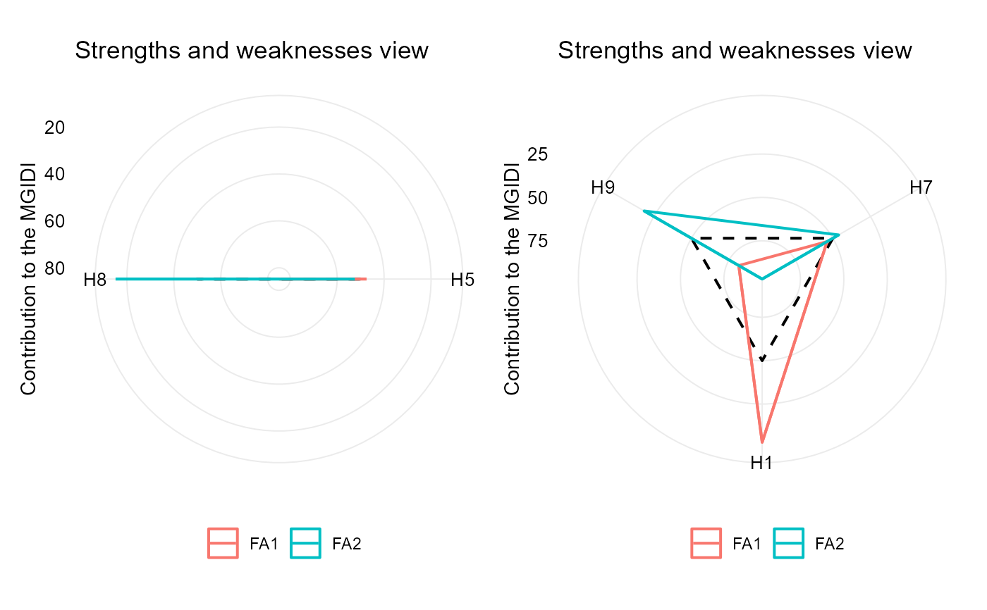
# plot the contribution of each factor on the MGIDI index
p1 <- plot(mgidi_ind, type = "contribution")
p2 <- plot(mgidi_ind2, type = "contribution")
p1 + p2
 # Positive desired gains for V1, V2 and V3
# Negative desired gains for V4
mgidi_ind3 <-
mgidi(mod,
ideotype = c("h, h, h, l"))
#>
#> -------------------------------------------------------------------------------
#> Principal Component Analysis
#> -------------------------------------------------------------------------------
#> # A tibble: 4 × 4
#> PC Eigenvalues `Variance (%)` `Cum. variance (%)`
#> <chr> <dbl> <dbl> <dbl>
#> 1 PC1 1.99 49.8 49.8
#> 2 PC2 1.01 25.2 75.0
#> 3 PC3 0.78 19.5 94.5
#> 4 PC4 0.22 5.51 100
#> -------------------------------------------------------------------------------
#> Factor Analysis - factorial loadings after rotation-
#> -------------------------------------------------------------------------------
#> # A tibble: 4 × 5
#> VAR FA1 FA2 Communality Uniquenesses
#> <chr> <dbl> <dbl> <dbl> <dbl>
#> 1 V1 0.57 0.19 0.37 0.63
#> 2 V2 -0.91 0.18 0.86 0.14
#> 3 V3 -0.81 -0.41 0.82 0.18
#> 4 V4 -0.1 -0.97 0.96 0.04
#> -------------------------------------------------------------------------------
#> Comunalit Mean: 0.7502531
#> -------------------------------------------------------------------------------
#> Selection differential
#> -------------------------------------------------------------------------------
#> # A tibble: 4 × 11
#> VAR Factor Xo Xs SD SDperc h2 SG SGperc sense goal
#> <chr> <chr> <dbl> <dbl> <dbl> <dbl> <dbl> <dbl> <dbl> <chr> <dbl>
#> 1 V1 FA1 103. 78.9 -24.3 -23.6 0.992 -24.2 -23.4 increase 0
#> 2 V2 FA1 102. 107. 4.98 4.87 0.993 4.94 4.83 increase 100
#> 3 V3 FA1 97.1 115. 18.2 18.8 0.979 17.9 18.4 increase 100
#> 4 V4 FA2 100. 69.1 -30.9 -30.9 0.989 -30.6 -30.6 decrease 100
#> ------------------------------------------------------------------------------
#> Selected genotypes
#> -------------------------------------------------------------------------------
#> H2 H10
#> -------------------------------------------------------------------------------
# }
# Positive desired gains for V1, V2 and V3
# Negative desired gains for V4
mgidi_ind3 <-
mgidi(mod,
ideotype = c("h, h, h, l"))
#>
#> -------------------------------------------------------------------------------
#> Principal Component Analysis
#> -------------------------------------------------------------------------------
#> # A tibble: 4 × 4
#> PC Eigenvalues `Variance (%)` `Cum. variance (%)`
#> <chr> <dbl> <dbl> <dbl>
#> 1 PC1 1.99 49.8 49.8
#> 2 PC2 1.01 25.2 75.0
#> 3 PC3 0.78 19.5 94.5
#> 4 PC4 0.22 5.51 100
#> -------------------------------------------------------------------------------
#> Factor Analysis - factorial loadings after rotation-
#> -------------------------------------------------------------------------------
#> # A tibble: 4 × 5
#> VAR FA1 FA2 Communality Uniquenesses
#> <chr> <dbl> <dbl> <dbl> <dbl>
#> 1 V1 0.57 0.19 0.37 0.63
#> 2 V2 -0.91 0.18 0.86 0.14
#> 3 V3 -0.81 -0.41 0.82 0.18
#> 4 V4 -0.1 -0.97 0.96 0.04
#> -------------------------------------------------------------------------------
#> Comunalit Mean: 0.7502531
#> -------------------------------------------------------------------------------
#> Selection differential
#> -------------------------------------------------------------------------------
#> # A tibble: 4 × 11
#> VAR Factor Xo Xs SD SDperc h2 SG SGperc sense goal
#> <chr> <chr> <dbl> <dbl> <dbl> <dbl> <dbl> <dbl> <dbl> <chr> <dbl>
#> 1 V1 FA1 103. 78.9 -24.3 -23.6 0.992 -24.2 -23.4 increase 0
#> 2 V2 FA1 102. 107. 4.98 4.87 0.993 4.94 4.83 increase 100
#> 3 V3 FA1 97.1 115. 18.2 18.8 0.979 17.9 18.4 increase 100
#> 4 V4 FA2 100. 69.1 -30.9 -30.9 0.989 -30.6 -30.6 decrease 100
#> ------------------------------------------------------------------------------
#> Selected genotypes
#> -------------------------------------------------------------------------------
#> H2 H10
#> -------------------------------------------------------------------------------
# }