Analyzing multienvironment trials using AMMI
Tiago Olivoto
2023-03-06
Source:vignettes/vignettes_ammi.Rmd
vignettes_ammi.RmdGetting started
In this section, we will use the data in data_ge. For
more information, please, see ?data_ge. Other data sets can
be used provided that the following columns are in the dataset:
environment, genotype, block/replicate and response variable(s). See the
section Rendering engine to know how HTML
tables were generated.
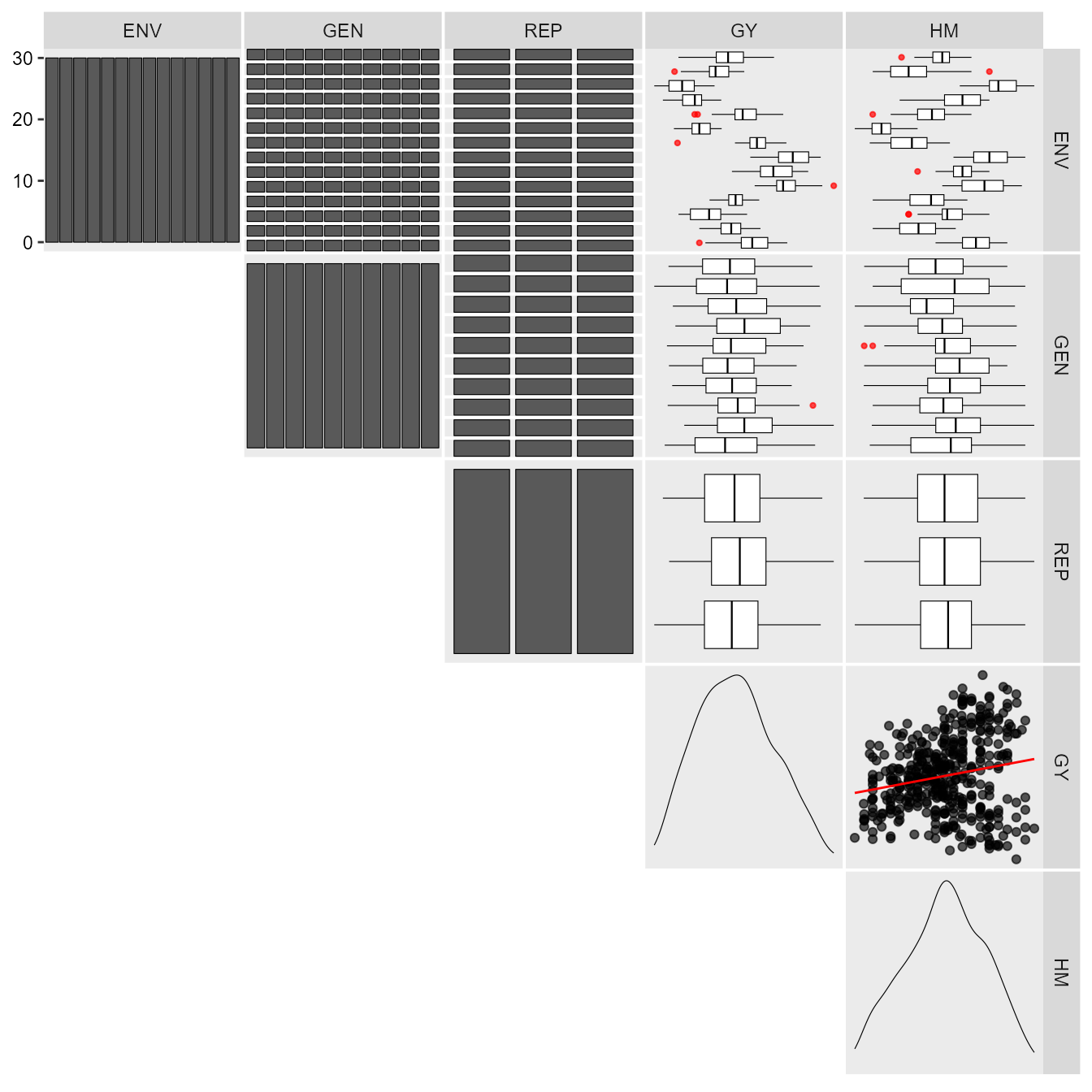
The first step is to inspect the data with the function
inspect().
print_table(insp)Individual and joint ANOVA
It is suggested to check if genotype-vs-environment interaction is
significant before proceeding with the AMMI analysis. A
within-environment ANOVA considering a fixed-effect model is computed
with the function anova_ind(). For each environment the
Mean Squares for block, genotypes and error are shown. Estimated F-value
and the probability error are also shown for block and genotype effects.
Some measures of experimental precision are calculated, namely,
coefficient of variation, \(CV =
(\sqrt{MS_{res}}/Mean) \times 100\); the heritability, \(h2 = (MS_{gen} - MS_{res})/MS_{gen}\), and
the accuracy of selection, \(As =
\sqrt{h2}\).
indiv <- anova_ind(data_ge, ENV, GEN, REP, GY)
# Evaluating trait GY |============================================| 100% 00:00:00
print_table(indiv$GY$individual)
The joint ANOVA is performed with the function
anova_joint().
library(metan)
joint <- anova_joint(data_ge, ENV, GEN, REP, GY, verbose = FALSE)
print_table(joint$GY$anova)
The genotype-vs-environment interaction was highly significant. So we’ll proceed with the AMMI analysis.
The AMMI model
The estimate of the response variable for the ith genotype in the jth environment using The Additive Main Effect and Multiplicative interaction (AMMI) model, is given as follows:
\[ {y_{ij}} = \mu + {\alpha_i} + {\tau_j} + \sum\limits_{k = 1}^p {{\lambda _k}{a_{ik}}} {t_{jk}} + {\rho _{ij}} + {\varepsilon _{ij}} \]
where \({\lambda_k}\) is the singular value for the k-th interaction principal component axis (IPCA); \(a_{ik}\) is the i-th element of the k-th eigenvector; \(t_{jk}\) is the jth element of the kth eigenvector. A residual \(\rho _{ij}\) remains, if not all p IPCA are used, where \(p \le min(g - 1; e - 1)\).
The AMMI model is fitted with the performs_ammi()
function. The first argument is the data, in our example
data_ge. The second argument (resp) is the
response variable to be analyzed. The function allow a single variable
(in this case GY) or a vector of response variables. The arguments
(gen, env, and rep) are the name
of the columns that contains the levels for genotypes, environments, and
replications, respectively. The last argument (verbose)
control if the code will run silently.
AMMI_model <- performs_ammi(data_ge,
                            env = ENV,
                            gen = GEN,
                            rep = REP,
                            resp = GY,
                            verbose = FALSE)
Note that using the arguments in the correct order, the model above may be fitted cleanly with:
AMMI_model <- performs_ammi(data_ge, ENV, GEN, REP, GY, verbose = FALSE)The AMMI table
The following comand creates the well-known ANOVA table for the AMMI model. Note that since
AMMI_model
# Variable GY
# ---------------------------------------------------------------------------
# AMMI analysis table
# ---------------------------------------------------------------------------
#       Source  Df     Sum Sq     Mean Sq   F value       Pr(>F) Proportion
# 1        ENV  13 279.573552 21.50565785 62.325457 0.000000e+00         NA
# 2   REP(ENV)  28   9.661516  0.34505416  3.568548 3.593191e-08         NA
# 3        GEN   9  12.995044  1.44389374 14.932741 2.190118e-19         NA
# 4    GEN:ENV 117  31.219565  0.26683389  2.759595 1.005191e-11         NA
# 5        PC1  21  10.749140  0.51186000  5.290000 0.000000e+00       34.4
# 6        PC2  19   9.923920  0.52231000  5.400000 0.000000e+00       31.8
# 7        PC3  17   4.039180  0.23760000  2.460000 1.400000e-03       12.9
# 8        PC4  15   3.073770  0.20492000  2.120000 9.600000e-03        9.8
# 9        PC5  13   1.446440  0.11126000  1.150000 3.176000e-01        4.6
# 10       PC6  11   0.932240  0.08475000  0.880000 5.606000e-01        3.0
# 11       PC7   9   0.566700  0.06297000  0.650000 7.535000e-01        1.8
# 12       PC8   7   0.362320  0.05176000  0.540000 8.037000e-01        1.2
# 13       PC9   5   0.125860  0.02517000  0.260000 9.345000e-01        0.4
# 14 Residuals 252  24.366674  0.09669315        NA           NA         NA
# 15     Total 536 389.035920  0.72581328        NA           NA         NA
#    Accumulated
# 1           NA
# 2           NA
# 3           NA
# 4           NA
# 5         34.4
# 6         66.2
# 7         79.2
# 8         89.0
# 9         93.6
# 10        96.6
# 11        98.4
# 12        99.6
# 13       100.0
# 14          NA
# 15          NA
# ---------------------------------------------------------------------------
# Scores for genotypes and environments
# ---------------------------------------------------------------------------
# # A tibble: 24 × 12
#    type  Code      Y      PC1      PC2      PC3      PC4      PC5      PC6
#    <chr> <chr> <dbl>    <dbl>    <dbl>    <dbl>    <dbl>    <dbl>    <dbl>
#  1 GEN   G1    2.604  0.3166  -0.04417 -0.03600 -0.06595 -0.3125   0.4272
#  2 GEN   G10   2.471 -1.001   -0.5718  -0.1652  -0.3309  -0.1243  -0.1064
#  3 GEN   G2    2.744  0.1390   0.1988  -0.7331   0.4735  -0.04816 -0.2841
#  4 GEN   G3    2.955  0.04340 -0.1028   0.2284   0.1769  -0.1270  -0.1400
#  5 GEN   G4    2.642 -0.3251   0.4782  -0.09073  0.1417  -0.1924   0.3550
#  6 GEN   G5    2.537 -0.3260   0.2461   0.2452   0.1794   0.4662   0.03315
#  7 GEN   G6    2.534 -0.09836  0.2429   0.5607   0.2377   0.05094 -0.1011
#  8 GEN   G7    2.741  0.2849   0.5871  -0.2068  -0.7085   0.2315  -0.08406
#  9 GEN   G8    3.004  0.4995  -0.1916   0.3191  -0.1676  -0.3261  -0.2886
# 10 GEN   G9    2.510  0.4668  -0.8427  -0.1217   0.06385  0.3819   0.1889
# # … with 14 more rows, and 3 more variables: PC7 <dbl>, PC8 <dbl>, PC9 <dbl>
Nine interaction principal component axis (IPCA) were fitted and four were significant at 5% probability error. Based on this result, the AMMI4 model would be the best model to predict the yielding of the genotypes in the studied environments.
Estimating the response variable based on significant IPCA axes
The response variable of a two-way table (for example, the yield of
m genotypes in n environments) may be estimated using
the S3 method predict() applyed to an object of class
waas. This estimation is based on the number of
multiplicative terms declared in the function. If
naxis = 1, the AMMI1 (with one multiplicative term) is used
for estimating the response variable. If
naxis = min(g - 1; e - 1), the AMMIF is fitted. A summary
of all possible AMMI models is presented below.
| Member of AMMI family | Espected response of the i-th genotype in the jth environment |
|---|---|
| AMMI0 | \(\hat{y}_{ij} = \bar{y}_{i.} + \bar{y}_{.j} - \bar{y}_{..}\) |
| AMMI1 | \(\hat{y}_{ij} = \bar{y}_{i.} + \bar{y}_{.j} - \bar{y}_{..} +\lambda_1 a_{i1}t_{j1}\) |
| AMMI2 | \(\hat{y}_{ij} = \bar{y}_{i.} + \bar{y}_{.j} - \bar{y}_{..} +\lambda_1 a_{i1}t_{j1}+\lambda_2 a_{i2}t_{j2}\) |
| … | |
| AMMIF | \(\hat{y}_{ij} = \bar{y}_{i.} + \bar{y}_{.j} - \bar{y}_{..} +\lambda_1 a_{i1}t_{j1}+\lambda_2 a_{i2}t_{j2}+...+\lambda_p a_{ip}t_{jp}\) |
Procedures based on postdictive success, such as Gollobs’s test (Gollob
1968) or predictive success, such as cross-validation (Piepho
1994) should be used to define the number of IPCA used for
estimating the response variable in AMMI analysis. This package provides
both. The waas() function compute traditional AMMI analysis
showing the number of significant axes according to Gollobs’s test. On
the other hand, cv_ammif() function provides
cross-validation of AMMI-model family, considering a completely
randomized design (CRD) or a randomized complete block design
(RCBD).
predicted <- predict(AMMI_model, naxis = 4)
print_table(predicted)
The following values are presented: ENV is the environment; GEN is the genotype; Y is the response variable; resOLS is the residual (\(\hat{z}_{ij}\)) estimated by the Ordinary Least Square (OLS), where \(\hat{z}_{ij} = y_{ij} - \bar{y}_{i.} - \bar{y}_{.j} + \bar{y}_{ij}\); Ypred is the predicted value by OLS (\(\hat{y}_{ij} = y_{ij} -\hat{z}_{ij}\)); ResAMMI is the residual estimated by the AMMI model (\(\hat{a}_{ij}\)) considering the number of multiplicative terms informed in the function (in this case 5), where \(\hat{a}_{ij} = \lambda_1\alpha_{i1}\tau_{j1}+...+\lambda_5\alpha_{i5}\tau_{j5}\); YpredAMMI is the predicted value by AMMI model \(\hat{ya}_{ij} = \bar{y}_{i.} + \bar{y}_{.j} - \bar{y}_{ij}+\hat{a}_{ij}\); and AMMI0 is the predicted value when no multiplicative terms are used, i.e., \(\hat{y}_{ij} = \bar{y}_{i.} + \bar{y}_{.j} - \bar{y}_{ij}\).
Estimating the WAAS index
The waas() function computes the Weighted Average of
Absolute Scores (Olivoto, Lúcio, Da silva, Marchioro, et al.
2019) considering (i) all principal component axes that were
significant (\(p < 0.05\) by
default); or (ii) declaring a specific number of axes to be used,
according to the following equation:
\[ WAAS_i = \sum_{k = 1}^{p} |IPCA_{ik} \times EP_k|/ \sum_{k = 1}^{p}EP_k \]
where \(WAAS_i\) is the weighted average of absolute scores of the ith genotype; \(PCA_{ik}\) is the score of the ith genotype in the kth IPCA; and \(EP_k\) is the explained variance of the kth IPCA for \(k = 1,2,..,p\), considering p the number of significant PCAs, or a declared number of PCAs. The following functions may be used to do that.
waas_index <- waas(data_ge, ENV, GEN, REP, GY, verbose = FALSE)Number of axes based on F-test
In this example only IPCAs with P-value < 0.05 will be
considered in the WAAS estimation. This is the default setting and the
model was already fitted and stored into
AMMI_model>GY>model.
print_table(waas_index$GY$model)The output generated by the waas() function shows the
following results: type, genotype (GEN) or environment
(ENV); Code, the code attributed to each level of the
factors; Y, the response variable (in this case the
grain yield); WAAS the weighted average of the absolute
scores, estimated with all PCA axes with P-value \(\le\) 0.05; PctWAAS and
PctResp that are the percentage values for the WAAS and
Y, respectively; OrResp and OrWAAS
that are the ranks attributed to the genotype and environment regarding
the Y or WAAS, respectively; WAASY is the weighted
average of absolute scores and response variable. In this case,
considering equal weights for PctResp and PctWAAS, the WAASY for G1 is
estimated by: \(WAAS_{G1} =
[(24.87\times50)+(91.83\times50)]/50+50 = 58.35\). Then the
OrWAASY is the rank for the WAASY value. The genotype
(or environment) with the largest WAASY value has the first ranked.
Number of axes declared manually
The second option to compute the WAAS is by manually declaring a
specific number of multiplicative terms. In this case, the number of
terms declared is used independently of its significance. Let us, for
the moment, assume that after a cross-validation procedure the AMMI7 was
the most predictively accurate AMMI model and the researcher will use
this model. The additional argument naxis in the function
waas is then used to overwrite the default chose of
significant terms.
waas_index2 <- data_ge %>%
  waas(ENV, GEN, REP, GY,
       naxis = 7, # Use 7 IPCA for computing WAAS
       verbose = FALSE)
The only difference in this output is that here we declared that seven IPCA axes should be used for computing the WAAS value. Thus, only the values of WAAS, OrWAAS, WAASY and OrWAASY may have significant changes.
Biplots
Provided that an object of class waas or
performs_ammi is available in the global environment, the
graphics may be obtained using the function plot_scores().
To do that, we will revisit the previusly fitted model
AMMI_model . Please, refer to plot_scores()
for more details.
biplot type 1: GY x PC1
a <- plot_scores(AMMI_model)
b <- plot_scores(AMMI_model,
                 col.gen = "black",
                 col.env = "gray70",
                 col.segm.env = "gray70",
                 axis.expand = 1.5,
                 plot_theme = theme_metan(grid = "both"))
arrange_ggplot(a, b, tag_levels = "a")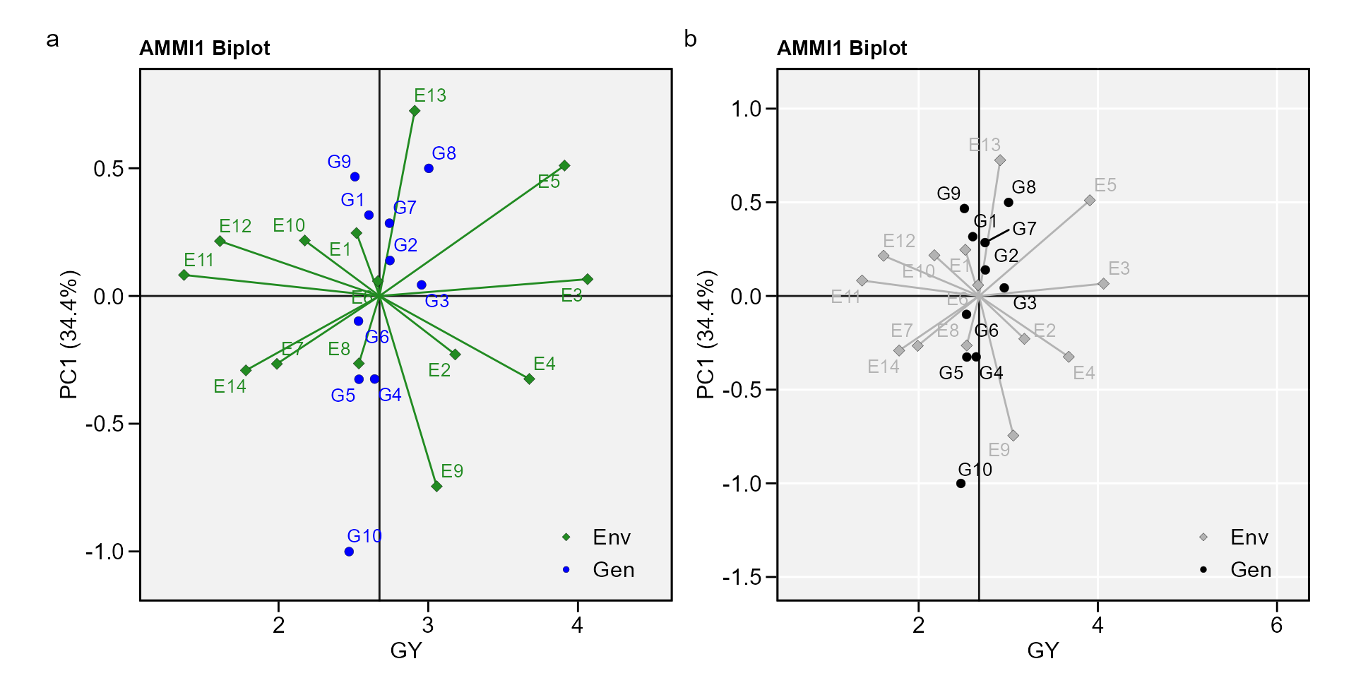
biplot type 2: PC1 x PC2
- PC1 x PC2 By default, IPCA1 is shown in the x axis and IPCA2 in the y axis.
c <- plot_scores(AMMI_model, type = 2)
d <- plot_scores(AMMI_model,
                 type = 2,
                 polygon = T,
                 col.segm.env = "transparent",
                 plot_theme = theme_metan_minimal())
arrange_ggplot(c, d, tag_levels = list(c("c", "d")))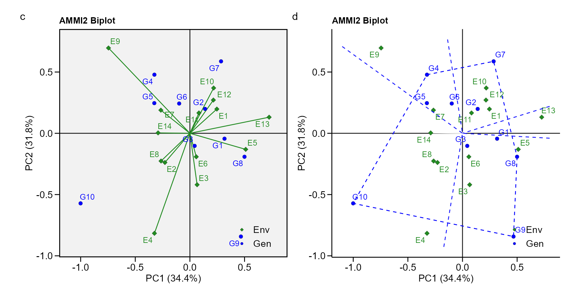
- Change the default option To create a biplot showin other IPCAs use
the arguments
firstandsecond. For example to produce a PC1 x PC3 biplot, usesecond = "PC3. A PC3 x PC4 biplot can be produced (provided that the model has at least four IPCAs) withfirst = "PC3"andsecond = "PC4"..
biplot type 3: GY x WAAS
The quadrants proposed by Olivoto, Lúcio, Da
silva, Marchioro, et al. (2019) in the following biplot represent
four classifications regarding the joint interpretation of mean
performance and stability. The genotypes or environments included in
quadrant I can be considered unstable genotypes or environments with
high discrimination ability, and with productivity below the grand mean.
In quadrant II are included unstable genotypes, although with
productivity above the grand mean. The environments included in this
quadrant deserve special attention since, in addition to providing high
magnitudes of the response variable, they present a good discrimination
ability. Genotypes within quadrant III have low productivity, but can be
considered stable due to the lower values of WAASB. The lower this
value, the more stable the genotype can be considered. The environments
included in this quadrant can be considered as poorly productive and
with low discrimination ability. The genotypes within the quadrant IV
are highly productive and broadly adapted due to the high magnitude of
the response variable and high stability performance (lower values of
WAASB). . To obtain this biplot must use an object of class
waas (in our example, waas_index).
e <- plot_scores(waas_index, type = 3)
f <- plot_scores(waas_index,
                 type = 3,
                 x.lab = "My custom x label",
                 size.shape.gen = 4, # Size of the shape for genotypes
                 col.gen = "gray50", # Color for genotypes
                 size.tex.gen = 4, # Size of the text for genotypes
                 col.alpha.env = 0, # Transparency of environment's point
                 x.lim = c(2.4, 3.1), # Limits of x axis
                 x.breaks = seq(2.4, 3.1, by = 0.1), # Markers of x axis
                 y.lim = c(0, 0.7))+
  ggplot2::ggtitle("WAASB vs GY plot", subtitle = "Zoom in genotypes' scores")
arrange_ggplot(e, f, tag_levels = list(c("e", "f")))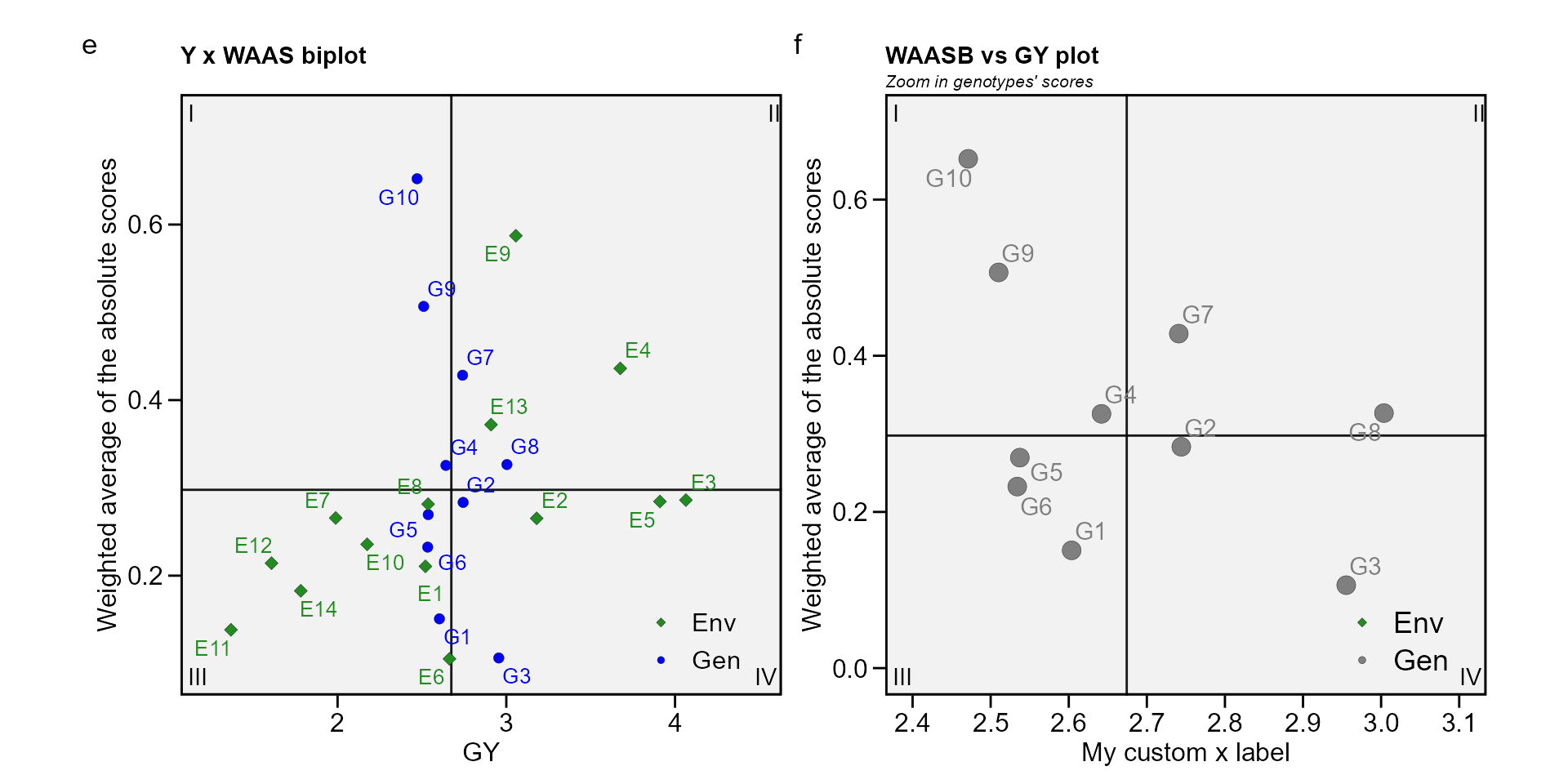
biplot type 4: nominal yield and environment IPCA1
g <- plot_scores(AMMI_model, type = 4)
h <- plot_scores(AMMI_model,
                 type = 4,
                 color = FALSE)
arrange_ggplot(g, h, tag_levels = list(c("g", "h")))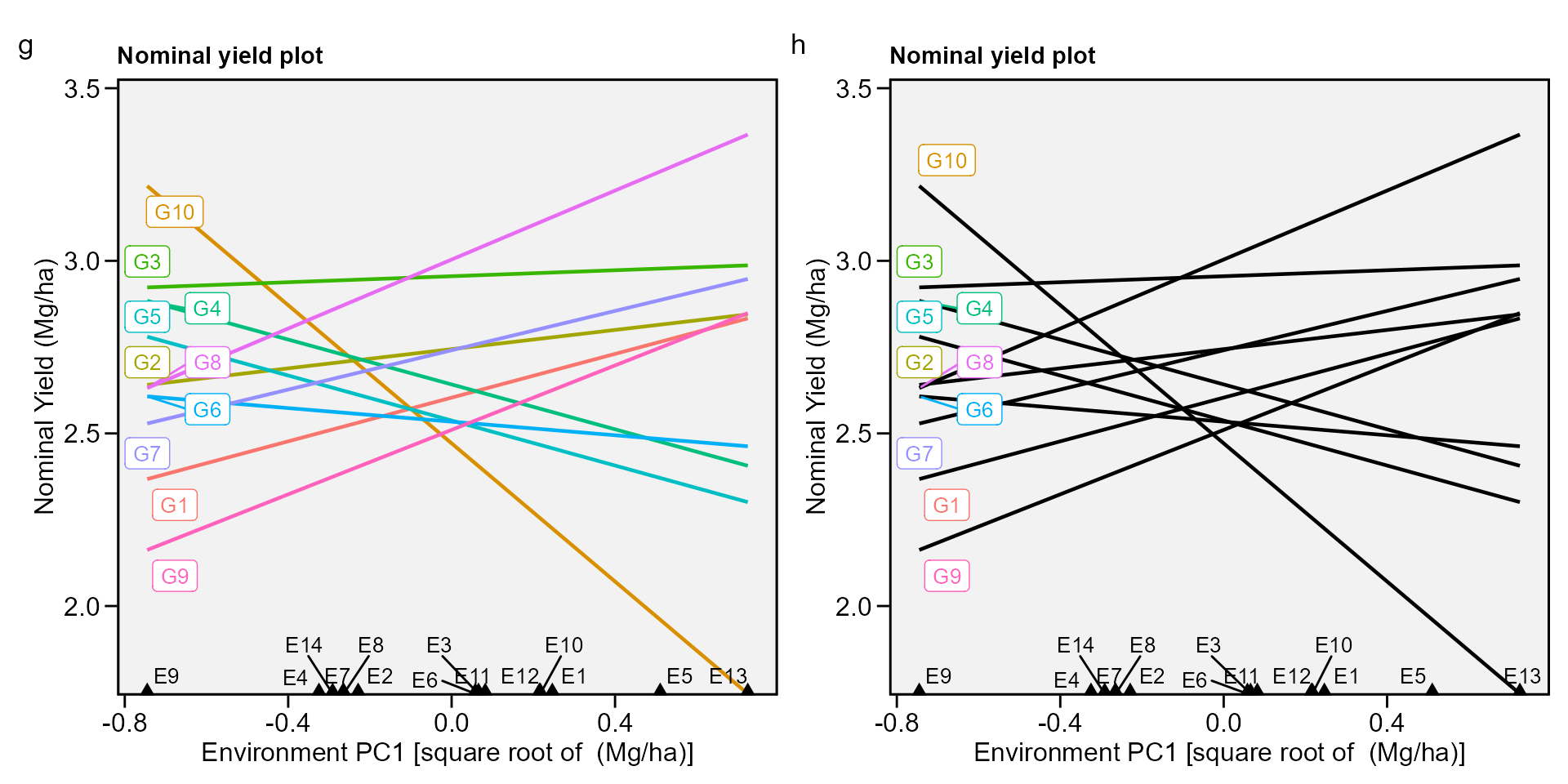
Simultaneous selection for mean performance and stability
The WAASY index (Olivoto, Lúcio, Da silva, Sari, et al. 2019) is used for genotype ranking considering both the stability (WAAS) and mean performance based on the following model:
\[ WAASY{_i} = \frac{{\left( {r{G_i} \times {\theta _Y}} \right) + \left( {r{W_i} \times {\theta _S}} \right)}}{{{\theta _Y} + {\theta _S}}} \]
where \(WAASY_i\) is the superiority index for the i-th genotype that weights between performance and stability; \(rG_i\) and \(rW_i\) are the rescaled values (0-100) for GY and WAASB, respectively; \(\theta _Y\) and \(\theta_S\) are the weights for GY and WAASB, respectively.
This index was also already computed and stored into AMMI_model>GY>model. An intuitively plot may be obtained by running
i <- plot_waasby(waas_index)
j <- plot_waasby(waas_index,
                 col.shape = c("gray20", "gray80"),
                 plot_theme = theme_metan(grid = "x"))
arrange_ggplot(i, j, tag_levels = list(c("i", "j")))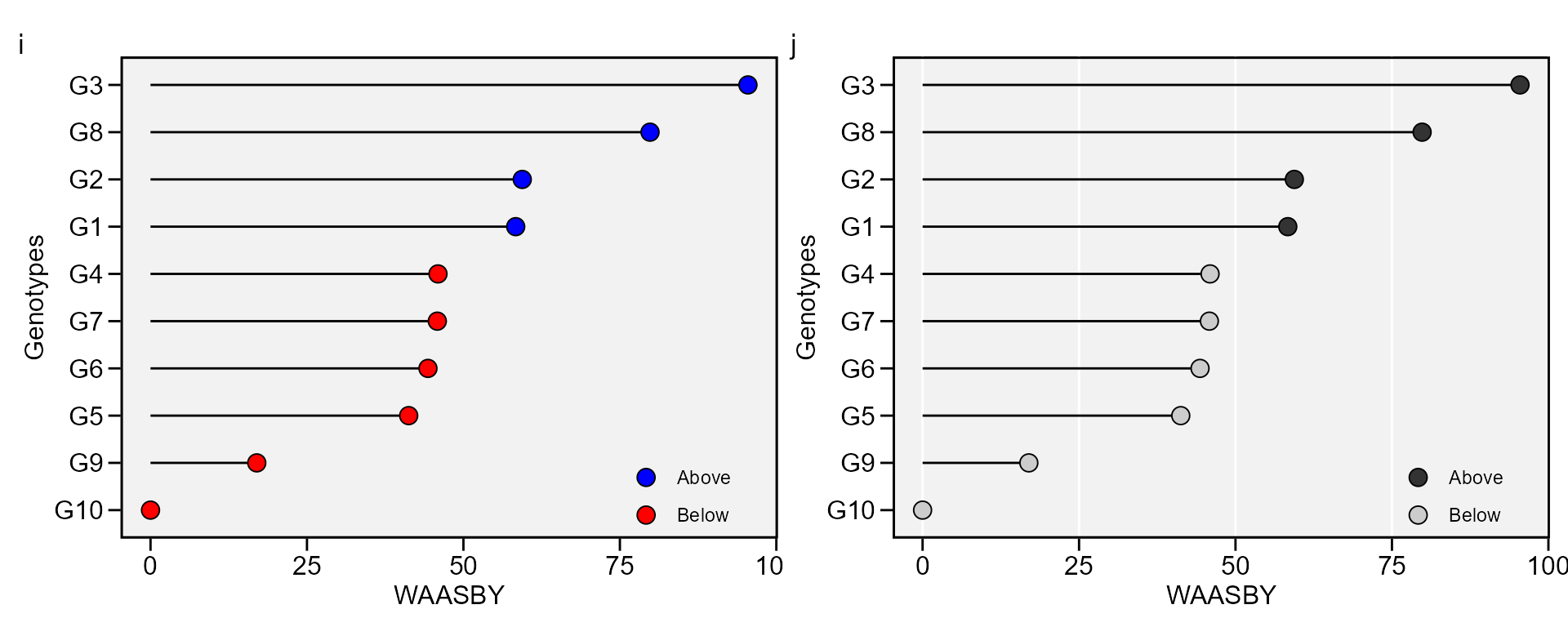
The values of WAASY in the plot above were computed considering equal
weights for mean performance and stability. Different weights may be
assigned using the wresp argument of the
waas() function.
Weighting the stability and mean performance
After fitting a model with the functions waas() or
waasb() it is possible to compute the superiority indexes
WAASY or WAASBY in different scenarios of weights for stability and mean
performance. The number of scenarios is defined by the arguments
increment. By default, twenty-one different scenarios are
computed. In this case, the the superiority index is computed
considering the following weights: stability (waasb or waas) = 100; mean
performance = 0. In other words, only stability is considered for
genotype ranking. In the next iteration, the weights becomes 95/5 (since
increment = 5). In the third scenario, the weights become 90/10, and so
on up to these weights become 0/100. In the last iteration, the genotype
ranking for WAASY or WAASBY matches perfectly with the ranks of the
response variable.
WAASratio <- wsmp(waas_index)Printing the model outputs
The genotype ranking for each scenario of WAASY/GY weight ratio is shown bellow
print_table(WAASratio$GY$hetcomb)In addition, the genotype ranking depending on the number of multiplicative terms used to estimate the WAAS index is also computed.
print_table(WAASratio$GY$hetdata)Plotting the heat map graphics
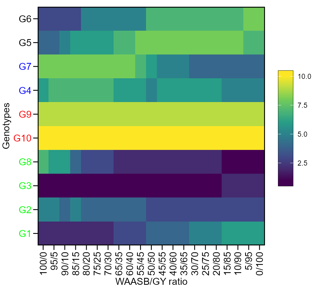
The first type of heatmap shows the genotype ranking depending on the number of principal component axes used for estimating the WAASB index. An euclidean distance-based dendrogram is used for grouping the genotype ranking for both genotypes and principal component axes. The second type of heatmap shows the genotype ranking depending on the WAASB/GY ratio. The ranks obtained with a ratio of 100/0 considers exclusively the stability for genotype ranking. On the other hand, a ratio of 0/100 considers exclusively the productivity for genotype ranking.
Ranks of genotypes depending on the number of PCA used to estimate the WAAS
plot(WAASratio, type = 1)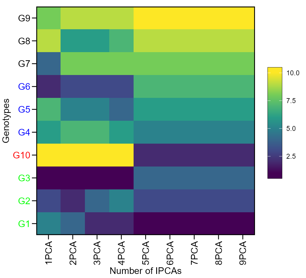
Getting model data
The function get_model_data() may be used to easily get
the data from a model fitted with the function waas(),
especially when more than one variables are used. Select helpers can be
used in the argument resp. See the example below.
waas_index_all <-
waas(data_ge2, ENV, GEN, REP,
     resp = everything()) %>%
 get_model_data(what = "WAASB")
print_table(waas_index_all)Other AMMI-based stability indexes
The following AMMI-based stability indexes may be computed using the
function AMMI_indexes():
- AMMI stability value, ASV, (Purchase, Hatting, and Deventer 2000).
\[ ASV = \sqrt {{{\left[ {\frac{{IPCA{1_{ss}}}}{{IPCA{2_{ss}}}} \times \left( {IPCA{1_{score}}} \right)} \right]}^2} + {{\left( {IPCA{2_{score}}} \right)}^2}} \]
- Sums of the absolute value of the IPCA scores
\[ SIP{C_i} = \sum\nolimits_{k = 1}^P {\left| {\mathop {\lambda }\nolimits_k^{0.5} {a_{ik}}} \right|} \]
- Averages of the squared eigenvector values
\[ E{V_i} = \sum\nolimits_{k = 1}^P {\mathop a\nolimits_{ik}^2 } /P \] described by Sneller, Kilgore-Norquest, and Dombek (1997), where P is the number of IPCA retained via F-tests;
- absolute value of the relative contribution of IPCAs to the interaction (Zali et al. 2012).
\[ Z{a_i} = \sum\nolimits_{k = 1}^P {{\theta _k}{a_{ik}}} \]
where \({\theta _k}\) is the percentage sum of squares explained by the k-th IPCA. Simultaneous selection indexes (ssi), are computed by summation of the ranks of the ASV, SIPC, EV and Za indexes and the ranks of the mean yields (Farshadfar 2008), which results in ssiASV, ssiSIPC, ssiEV, and ssiZa, respectively.
The AMMI_index() function has two arguments. The first
(x) is the model, which must be an object of the class waas
or performs_ammi. The second, (order.y) is the order for
ranking the response variable. By default, it is set to NULL, which
means that the response variable is ordered in descending order. If
x is a list with more than one variable,
order.y must be a vector of the same length of x. Each
element of the vector must be one of the “h” or “l”. If “h” is used, the
response variable will be ordered from maximum to minimum. If “l” is
used then the response variable will be ordered from minimum to maximum.
We will use the previously fitted model AMMI_model to
compute the AMMI-based stability indexes.
stab_indexes <- AMMI_indexes(AMMI_model)
# Warning in AMMI_indexes(AMMI_model): `AMMI_indexes()` is deprecated as of metan
# 1.16.0. use `ammi_indexes()` instead.
print_table(stab_indexes$GY)
AMMI model for unbalanced data
Singular Value Decomposition requires a complete two-way table (i.e.,
all genotypes in all environments). Sometimes (for several reasons), a
complete two-way table cannot be obtained in a multi-environment trial.
metan offers an option to impute the missing cells of the
two-way table using Expectation-Maximization algorithms. If an
incomplete two-way table is identified in performs_ammi() a
warning is issued, impute_missing_val() is called
internally and the missing value(s) is(are) imputed using a low-rank
Singular Value Decomposition approximation estimated by the
Expectation-Maximization algorithm. The algorithm will (i) initialize
all NA values to the column means; (ii) compute the first axis terms of
the SVD of the completed matrix; (iii) replace the previously missing
values with their approximations from the SVD; (iv) iterate steps 2
through 3 until convergence or a maximum number of iterations be
achieved.
As an example we will run the AMMI model by omiting H2
from E1 in `data_ge2.
miss_val <-
  data_ge2 %>%
  remove_rows(4:6) %>%
  droplevels()

mod_miss <-
  performs_ammi(miss_val, ENV, GEN, REP, PH)
# ----------------------------------------------
# Convergence information
# ----------------------------------------------
# Number of iterations: 23
# Final RMSE: 6.007683e-11
# Number of axis: 1
# Convergence: TRUE
# ----------------------------------------------
# Warning: Data imputation used to fill the GxE matrix
# variable PH
# ---------------------------------------------------------------------------
# AMMI analysis table
# ---------------------------------------------------------------------------
#     Source  Df Sum Sq Mean Sq F value   Pr(>F) Proportion Accumulated
#        ENV   3  6.952  2.3173 117.463 5.92e-07         NA          NA
#   REP(ENV)   8  0.158  0.0197   0.863 5.51e-01         NA          NA
#        GEN  12  2.470  0.2058   9.000 3.03e-11         NA          NA
#    GEN:ENV  35  5.286  0.1510   6.603 1.39e-13         NA          NA
#        PC1  14  4.413  0.3152  13.780 0.00e+00       83.4        83.4
#        PC2  12  0.588  0.0490   2.140 2.12e-02       11.1        94.5
#        PC3  10  0.290  0.0290   1.270 2.59e-01        5.5       100.0
#  Residuals  94  2.150  0.0229      NA       NA         NA          NA
#      Total 188 22.306  0.1187      NA       NA         NA          NA
# ---------------------------------------------------------------------------
#
# All variables with significant (p < 0.05) genotype-vs-environment interaction
# Done!
p1 <- plot_scores(mod_miss, type = 2, title = FALSE)

mod_comp <-
  data_ge2 %>%
  performs_ammi(ENV, GEN, REP, PH)
# variable PH
# ---------------------------------------------------------------------------
# AMMI analysis table
# ---------------------------------------------------------------------------
#     Source  Df Sum Sq Mean Sq F value   Pr(>F) Proportion Accumulated
#        ENV   3  7.719  2.5728 127.913 4.25e-07         NA          NA
#   REP(ENV)   8  0.161  0.0201   0.897 5.22e-01         NA          NA
#        GEN  12  1.865  0.1554   6.929 6.89e-09         NA          NA
#    GEN:ENV  36  5.397  0.1499   6.686 5.01e-14         NA          NA
#        PC1  14  4.466  0.3190  14.230 0.00e+00       82.8        82.8
#        PC2  12  0.653  0.0545   2.430 8.40e-03       12.1        94.9
#        PC3  10  0.277  0.0277   1.240 2.76e-01        5.1       100.0
#  Residuals  96  2.153  0.0224      NA       NA         NA          NA
#      Total 191 22.692  0.1188      NA       NA         NA          NA
# ---------------------------------------------------------------------------
#
# All variables with significant (p < 0.05) genotype-vs-environment interaction
# Done!
p2 <- plot_scores(mod_comp, type = 2, title = FALSE)

arrange_ggplot(p1, p2, tag_levels = list(c("Missing data", "Complete data")))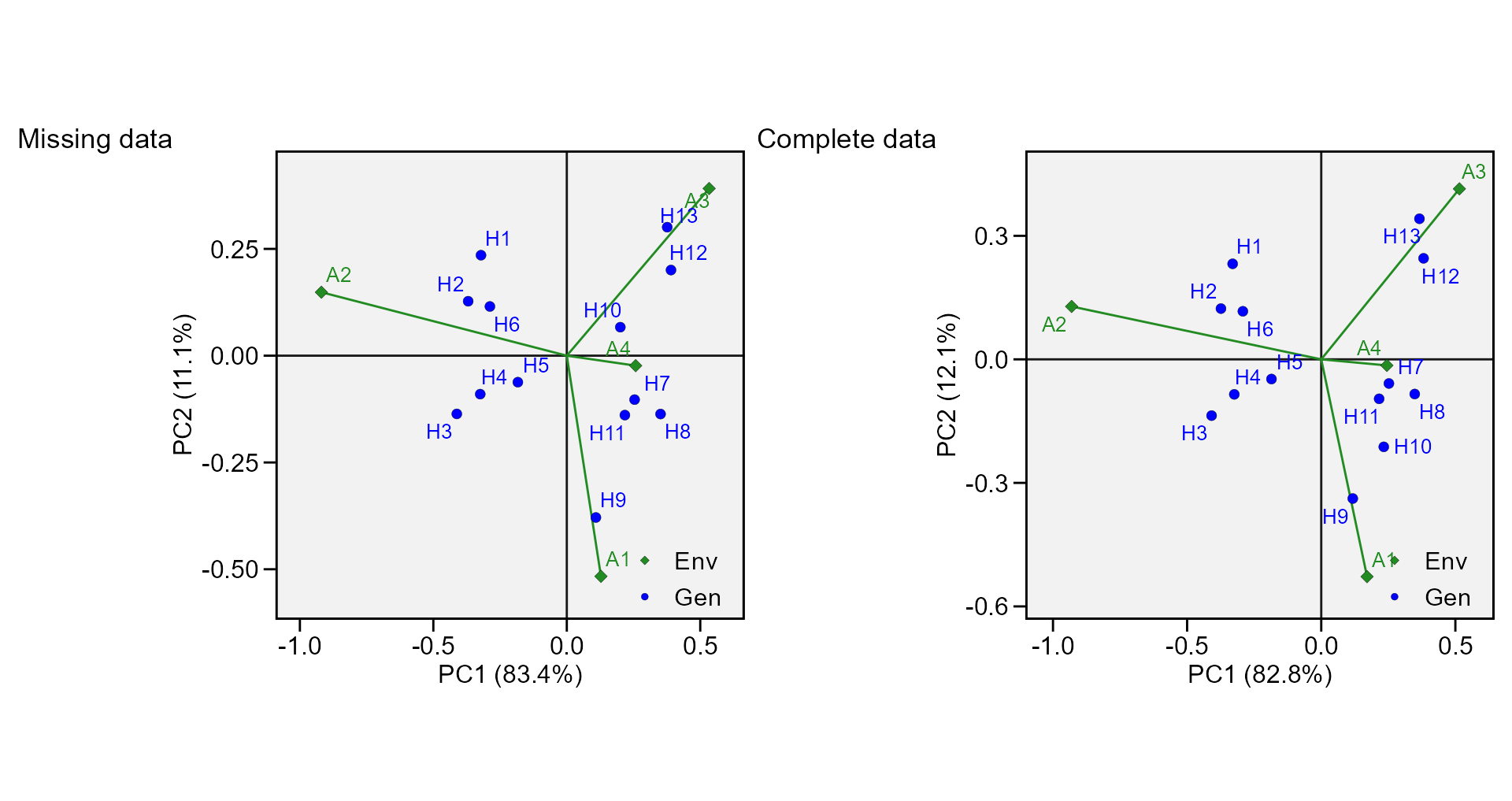
Rendering engine
This vignette was built with pkgdown. All tables were produced
with the package DT using the
following function.
library(DT) # Used to make the tables
# Function to make HTML tables
print_table <- function(table, rownames = FALSE, digits = 3, ...){
datatable(table, rownames = rownames, extensions = 'Buttons',
          options = list(scrollX = TRUE,
                         dom = '<<t>Bp>',
                         buttons = c('copy', 'excel', 'pdf', 'print')), ...) %>%
    formatSignif(columns = c(as.numeric(which(sapply(table, class) == "numeric"))), digits = digits)}