![[Stable]](figures/lifecycle-stable.svg)
Plot scores of genotypes and environments in different graphical interpretations.
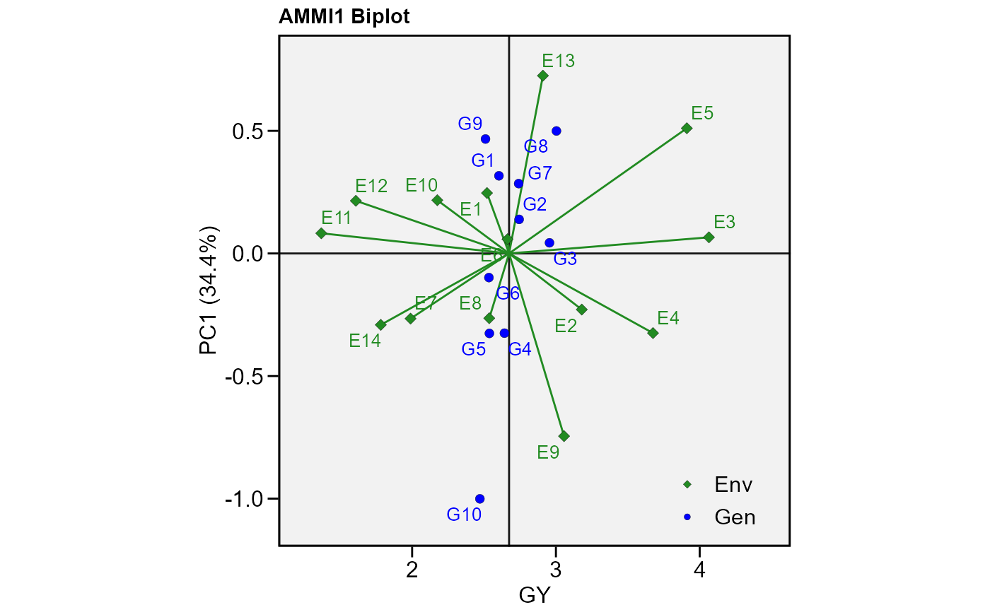
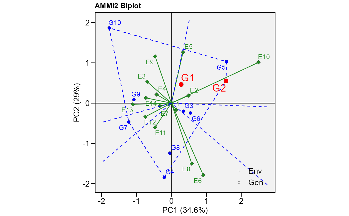
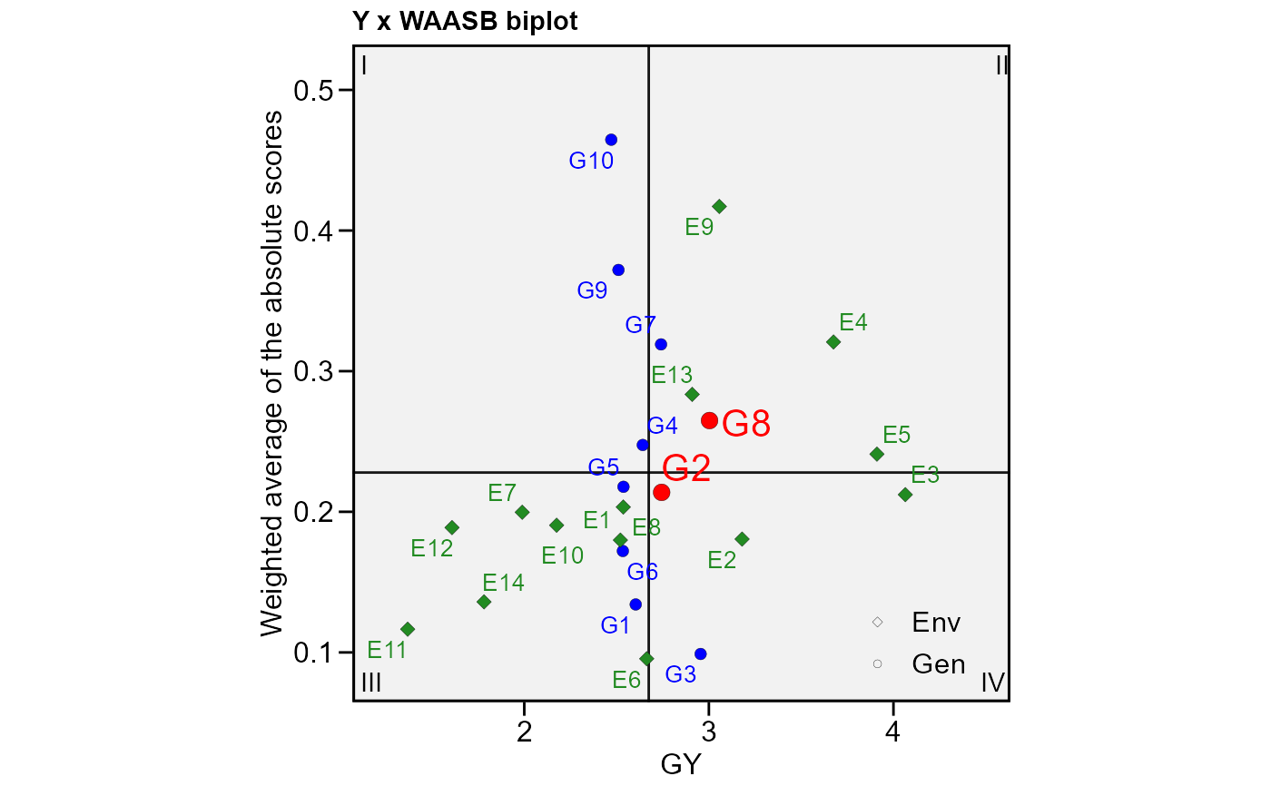
Biplots type 1 and 2 are well known in AMMI analysis. In the plot type 3, the scores of both genotypes and environments are plotted considering the response variable and the WAASB, an stability index that considers all significant principal component axis of traditional AMMI models or all principal component axis estimated with BLUP-interaction effects (Olivoto et al. 2019). Plot type 4 may be used to better understand the well known 'which-won-where' pattern, facilitating the recommendation of appropriate genotypes targeted for specific environments, thus allowing the exploitation of narrow adaptations.
Usage
plot_scores(
  x,
  var = 1,
  type = 1,
  first = "PC1",
  second = "PC2",
  repel = TRUE,
  repulsion = 1,
  max_overlaps = 20,
  polygon = FALSE,
  title = TRUE,
  plot_theme = theme_metan(),
  axis.expand = 1.1,
  x.lim = NULL,
  y.lim = NULL,
  x.breaks = waiver(),
  y.breaks = waiver(),
  x.lab = NULL,
  y.lab = NULL,
  shape.gen = 21,
  shape.env = 23,
  size.shape.gen = 2.2,
  size.shape.env = 2.2,
  size.bor.tick = 0.1,
  size.tex.lab = 12,
  size.tex.gen = 3.5,
  size.tex.env = 3.5,
  size.line = 0.5,
  size.segm.line = 0.5,
  col.bor.gen = "black",
  col.bor.env = "black",
  col.line = "black",
  col.gen = "blue",
  col.env = "forestgreen",
  col.alpha.gen = 1,
  col.alpha.env = 1,
  col.segm.gen = transparent_color(),
  col.segm.env = "forestgreen",
  highlight = NULL,
  col.highlight = "red",
  col.alpha.highlight = 1,
  size.tex.highlight = 5.5,
  size.shape.highlight = 3.2,
  leg.lab = c("Env", "Gen"),
  line.type = "solid",
  line.alpha = 0.9,
  resolution = deprecated(),
  file.type = "png",
  export = FALSE,
  file.name = NULL,
  width = 8,
  height = 7,
  color = TRUE,
  ...
)
Arguments
- x
An object fitted with the functions
performs_ammi(),waas(),waas_means(), orwaasb().- var
The variable to plot. Defaults to
var = 1the first variable ofx.- type
type of biplot to produce
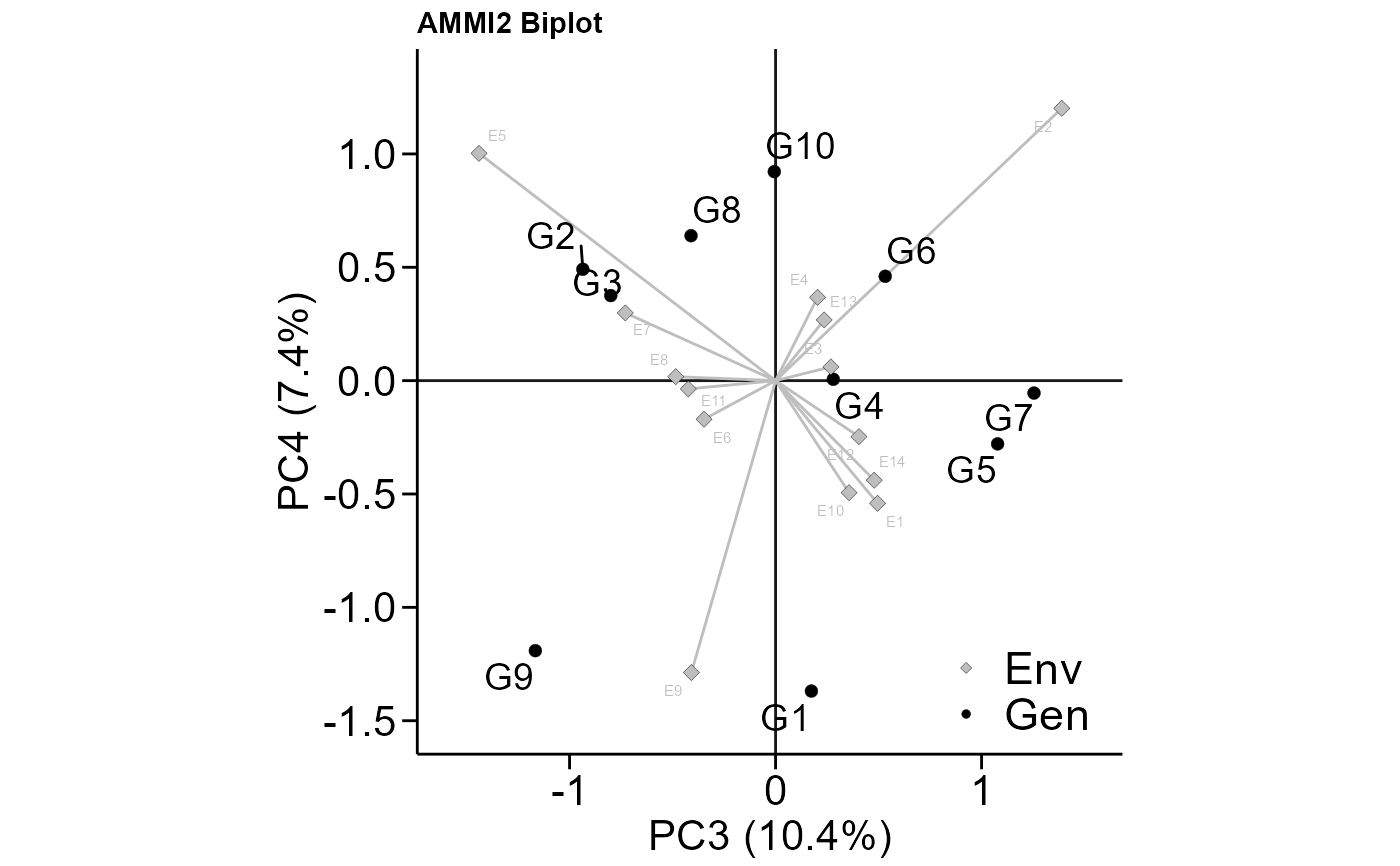
type = 1The default. Produces an AMMI1 biplot (Y x PC1) to make inferences related to stability and productivity.type = 2Produces an AMMI2 biplot (PC1 x PC2) to make inferences related to the interaction effects. Use the argumentsfirstorsecondto change the default IPCA shown in the plot.type = 3Valid for objects of classwaasorwaasb, produces a biplot showing the GY x WAASB.type = 4Produces a plot with the Nominal yield x Environment PC.
- first, second
The IPCA to be shown in the first (x) and second (y) axis. By default, IPCA1 is shown in the
xaxis and IPCA2 in theyaxis. For example, usesecond = "PC3"to shown the IPCA3 in theyaxis.- repel
If
TRUE(default), the text labels repel away from each other and away from the data points.- repulsion
Force of repulsion between overlapping text labels. Defaults to
1.- max_overlaps
Exclude text labels that overlap too many things. Defaults to 20.
- polygon
Logical argument. If
TRUE, a polygon is drawn whentype = 2.- title
Logical values (Defaults to
TRUE) to include automatically generated titles- plot_theme
The graphical theme of the plot. Default is
plot_theme = theme_metan(). For more details, seeggplot2::theme().- axis.expand
Multiplication factor to expand the axis limits by to enable fitting of labels. Default is
1.1.- x.lim, y.lim
The range of x and y axes, respectively. Default is
NULL(maximum and minimum values of the data set). New values can be inserted asx.lim = c(x.min, x.max)ory.lim = c(y.min, y.max).- x.breaks, y.breaks
The breaks to be plotted in the x and y axes, respectively. Defaults to
waiver()(automatic breaks). New values can be inserted, for example, asx.breaks = c(0.1, 0.2, 0.3)orx.breaks = seq(0, 1, by = 0.2)- x.lab, y.lab
The label of x and y axes, respectively. Defaults to
NULL, i.e., each plot has a default axis label. New values can be inserted asx.lab = 'my label'.- shape.gen, shape.env
The shape for genotypes and environments indication in the biplot. Default is
21(circle) for genotypes and23(diamond) for environments. Values must be between21-25:21(circle),22(square),23(diamond),24(up triangle), and25(low triangle).- size.shape.gen, size.shape.env
The size of the shapes for genotypes and environments respectively. Defaults to
2.2.- size.bor.tick
The size of tick of shape. Default is
0.1. The size of the shape will bemax(size.shape.gen, size.shape.env) + size.bor.tick- size.tex.lab, size.tex.gen, size.tex.env
The size of the text for axis labels (Defaults to 12), genotypes labels, and environments labels (Defaults to 3.5).
- size.line
The size of the line that indicate the means in the biplot. Default is
0.5.- size.segm.line
The size of the segment that start in the origin of the biplot and end in the scores values. Default is
0.5.- col.bor.gen, col.bor.env
The color of the shape's border for genotypes and environments, respectively.
- col.line
The color of the line that indicate the means in the biplot. Default is
'gray'- col.gen, col.env
The shape color for genotypes (Defaults to
'blue') and environments ('forestgreen'). Must be length one or a vector of colors with the same length of the number of genotypes/environments.- col.alpha.gen, col.alpha.env
The alpha value for the color for genotypes and environments, respectively. Defaults to
NA. Values must be between0(full transparency) to1(full color).- col.segm.gen, col.segm.env
The color of segment for genotypes (Defaults to
transparent_color()) and environments (Defaults to 'forestgreen'), respectively. Valid arguments for plots withtype = 1ortype = 2graphics.- highlight
Genotypes/environments to be highlight in the plot. Defaults to
NULL.- col.highlight
The color for shape/labels when a value is provided in
highlight.Defaults to"red".- col.alpha.highlight
The alpha value for the color of the highlighted genotypes. Defaults to
1.- size.tex.highlight
The size of the text for the highlighted genotypes. Defaults to
5.5.- size.shape.highlight
The size of the shape for the highlighted genotypes. Defaults to
3.2.- leg.lab
The labs of legend. Default is
GenandEnv.- line.type
The type of the line that indicate the means in the biplot. Default is
'solid'. Other values that can be attributed are:'blank', no lines in the biplot,'dashed', 'dotted', 'dotdash', 'longdash', and 'twodash'.- line.alpha
The alpha value that combine the line with the background to create the appearance of partial or full transparency. Default is
0.4. Values must be between '0' (full transparency) to '1' (full color).- resolution
deprecated
- file.type
The type of file to be exported. Currently recognises the extensions eps/ps, tex, pdf, jpeg, tiff, png (default), bmp, svg and wmf (windows only).
- export
Export (or not) the plot. Default is
FALSE. IfTRUE, calls theggplot2::ggsave()function.- file.name
The name of the file for exportation, default is
NULL, i.e. the files are automatically named.- width
The width 'inch' of the plot. Default is
8.- height
The height 'inch' of the plot. Default is
7.- color
Should type 4 plot have colors? Default to
TRUE.- ...
Currently not used.
References
Olivoto, T., A.D.C. L\'ucio, J.A.G. da silva, V.S. Marchioro, V.Q. de Souza, and E. Jost. 2019. Mean performance and stability in multi-environment trials I: Combining features of AMMI and BLUP techniques. Agron. J. 111:2949-2960. doi:10.2134/agronj2019.03.0220
Author
Tiago Olivoto tiagoolivoto@gmail.com
Examples
# \donttest{
library(metan)
# AMMI model
model <- waas(data_ge,
env = ENV,
gen = GEN,
rep = REP,
resp = everything())
#> variable GY
#> ---------------------------------------------------------------------------
#> AMMI analysis table
#> ---------------------------------------------------------------------------
#> Source Df Sum Sq Mean Sq F value Pr(>F) Proportion Accumulated
#> ENV 13 279.574 21.5057 62.33 0.00e+00 NA NA
#> REP(ENV) 28 9.662 0.3451 3.57 3.59e-08 NA NA
#> GEN 9 12.995 1.4439 14.93 2.19e-19 NA NA
#> GEN:ENV 117 31.220 0.2668 2.76 1.01e-11 NA NA
#> PC1 21 10.749 0.5119 5.29 0.00e+00 34.4 34.4
#> PC2 19 9.924 0.5223 5.40 0.00e+00 31.8 66.2
#> PC3 17 4.039 0.2376 2.46 1.40e-03 12.9 79.2
#> PC4 15 3.074 0.2049 2.12 9.60e-03 9.8 89.0
#> PC5 13 1.446 0.1113 1.15 3.18e-01 4.6 93.6
#> PC6 11 0.932 0.0848 0.88 5.61e-01 3.0 96.6
#> PC7 9 0.567 0.0630 0.65 7.53e-01 1.8 98.4
#> PC8 7 0.362 0.0518 0.54 8.04e-01 1.2 99.6
#> PC9 5 0.126 0.0252 0.26 9.34e-01 0.4 100.0
#> Residuals 252 24.367 0.0967 NA NA NA NA
#> Total 536 389.036 0.7258 NA NA NA NA
#> ---------------------------------------------------------------------------
#>
#> variable HM
#> ---------------------------------------------------------------------------
#> AMMI analysis table
#> ---------------------------------------------------------------------------
#> Source Df Sum Sq Mean Sq F value Pr(>F) Proportion Accumulated
#> ENV 13 5710.32 439.255 57.22 1.11e-16 NA NA
#> REP(ENV) 28 214.93 7.676 2.70 2.20e-05 NA NA
#> GEN 9 269.81 29.979 10.56 7.41e-14 NA NA
#> GEN:ENV 117 1100.73 9.408 3.31 1.06e-15 NA NA
#> PC1 21 381.13 18.149 6.39 0.00e+00 34.6 34.6
#> PC2 19 319.43 16.812 5.92 0.00e+00 29.0 63.6
#> PC3 17 114.26 6.721 2.37 2.10e-03 10.4 74.0
#> PC4 15 81.96 5.464 1.92 2.18e-02 7.4 81.5
#> PC5 13 68.11 5.240 1.84 3.77e-02 6.2 87.7
#> PC6 11 59.07 5.370 1.89 4.10e-02 5.4 93.0
#> PC7 9 46.69 5.188 1.83 6.33e-02 4.2 97.3
#> PC8 7 26.65 3.808 1.34 2.32e-01 2.4 99.7
#> PC9 5 3.41 0.682 0.24 9.45e-01 0.3 100.0
#> Residuals 252 715.69 2.840 NA NA NA NA
#> Total 536 9112.21 17.000 NA NA NA NA
#> ---------------------------------------------------------------------------
#>
#> All variables with significant (p < 0.05) genotype-vs-environment interaction
#> Done!
# GY x PC1 for variable GY (default plot)
plot_scores(model)
 # PC1 x PC2 (variable HM)
#
plot_scores(model,
polygon = TRUE, # Draw a convex hull polygon
var = "HM", # or var = 2 to select variable
highlight = c("G1", "G2"), # Highlight genotypes 2 and 3
type = 2) # type of biplot
# PC1 x PC2 (variable HM)
#
plot_scores(model,
polygon = TRUE, # Draw a convex hull polygon
var = "HM", # or var = 2 to select variable
highlight = c("G1", "G2"), # Highlight genotypes 2 and 3
type = 2) # type of biplot
 # PC3 x PC4 (variable HM)
# Change size of plot fonts and colors
# Minimal theme
plot_scores(model,
var = "HM",
type = 2,
first = "PC3",
second = "PC4",
col.gen = "black",
col.env = "gray",
col.segm.env = "gray",
size.tex.gen = 5,
size.tex.env = 2,
size.tex.lab = 16,
plot_theme = theme_metan_minimal())
# PC3 x PC4 (variable HM)
# Change size of plot fonts and colors
# Minimal theme
plot_scores(model,
var = "HM",
type = 2,
first = "PC3",
second = "PC4",
col.gen = "black",
col.env = "gray",
col.segm.env = "gray",
size.tex.gen = 5,
size.tex.env = 2,
size.tex.lab = 16,
plot_theme = theme_metan_minimal())
 # WAASB index
waasb_model <- waasb(data_ge, ENV, GEN, REP, GY)
#> Evaluating trait GY |============================================| 100% 00:00:02
#> Method: REML/BLUP
#> Random effects: GEN, GEN:ENV
#> Fixed effects: ENV, REP(ENV)
#> Denominador DF: Satterthwaite's method
#> ---------------------------------------------------------------------------
#> P-values for Likelihood Ratio Test of the analyzed traits
#> ---------------------------------------------------------------------------
#> model GY
#> COMPLETE NA
#> GEN 1.11e-05
#> GEN:ENV 2.15e-11
#> ---------------------------------------------------------------------------
#> All variables with significant (p < 0.05) genotype-vs-environment interaction
# GY x WAASB
# Highlight genotypes 2 and 8
plot_scores(waasb_model,
type = 3,
highlight = c("G2", "G8"))
# WAASB index
waasb_model <- waasb(data_ge, ENV, GEN, REP, GY)
#> Evaluating trait GY |============================================| 100% 00:00:02
#> Method: REML/BLUP
#> Random effects: GEN, GEN:ENV
#> Fixed effects: ENV, REP(ENV)
#> Denominador DF: Satterthwaite's method
#> ---------------------------------------------------------------------------
#> P-values for Likelihood Ratio Test of the analyzed traits
#> ---------------------------------------------------------------------------
#> model GY
#> COMPLETE NA
#> GEN 1.11e-05
#> GEN:ENV 2.15e-11
#> ---------------------------------------------------------------------------
#> All variables with significant (p < 0.05) genotype-vs-environment interaction
# GY x WAASB
# Highlight genotypes 2 and 8
plot_scores(waasb_model,
type = 3,
highlight = c("G2", "G8"))
 # }
# }