Parametric and non-parametric stability statistics
Tiago Olivoto
2023-03-06
Source:vignettes/vignettes_stability.Rmd
vignettes_stability.RmdGetting started
In this section, we will use the data in data_ge and
data_ge2. For more information see ?data_ge
and ?data_ge2, respectively. Other data sets can be used
provided that the following columns are in the data_ge: environment,
genotype, block/replicate and response variable(s).
See the section Rendering engine to know how HTML tables were generated.
Genotype-environment performance
The function ge_plot() may be used to visualize the
genotype’s performance across the environments.
library(metan)
a <- ge_plot(data_ge, ENV, GEN, GY)
b <- ge_plot(data_ge, ENV, GEN, GY) + ggplot2::coord_flip()
arrange_ggplot(a, b, tag_levels = "a")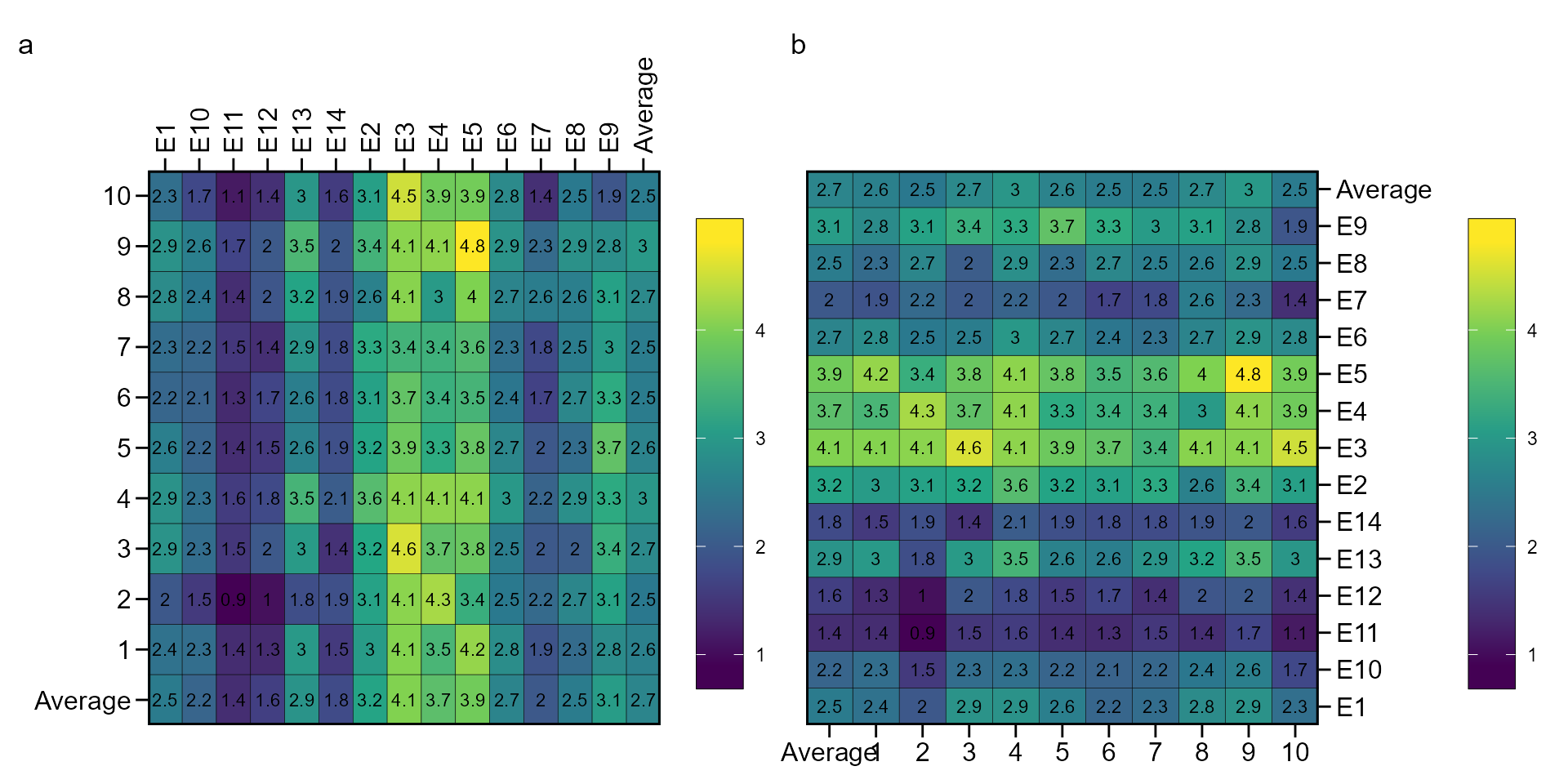
To identify the winner genotype within each environment, we can use
the function ge_winners().
ge_winners(data_ge2, ENV, GEN, resp = everything()) %>% print_table()Or get the genotype ranking within each environment.
ge_winners(data_ge2, ENV, GEN, resp = everything(), type = "ranks") %>%
  print_table()
For more details about the trials, we can use
ge_details()
ge_details(data_ge2, ENV, GEN, resp = everything()) %>%
  print_table()
Within-environment analysis of variance
The function anova_ind() can be used to compute an
within-environment analysis of variance. Environment with values in blue
had a significant (p < 0.05) genotype effect.
ind <- anova_ind(data_ge, ENV, GEN, REP, GY)
# Evaluating trait GY |============================================| 100% 00:00:00
print_table(ind$GY$individual)
Genotype-by-environment means
The function make_mat() can be used to produce a two-way
table for the genotype-environment means.
Genotype-by-environment interaction effects
The function ge_effects() is used to compute the
genotype-environment effects.
ge_ef <- ge_effects(data_ge, ENV, GEN, GY)
print_table(ge_ef$GY)
Genotype plus Genotype-by-environment effects
To obtain the genotype plus genotype-environment effects, we can use
the argument type = "gge" in the function
ge_effects().
gge_ef <- ge_effects(data_ge, ENV, GEN, GY, type = "gge")
print_table(gge_ef$GY)
Clustering tester locations
The function ge_cluster() computes a cluster analysis
for grouping environments based on its similarities using an Euclidean
distance based on standardized data. Line means are divided by the
phenotypic standard error of the relevant environment after its mean has
been subtracted. By standardizing the data each environment will have a
mean of zero and unit variance, and the effect of variability in
phenotypic variance (as well as the mean) should be reduced (Fox and
Rosielle 1982).
d1 <- ge_cluster(data_ge, ENV, GEN, GY, nclust = 4)
plot(d1, nclust = 4)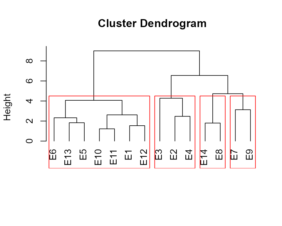
The function env_dissimilarity() computes the
dissimilarity between test environment using:
The partition of the partition of the mean square of the genotype-environment interaction (MS_GE) into single (S) and complex (C) parts, according to Robertson (1959), where \(S = \frac{1}{2}(\sqrt{Q_1}-\sqrt{Q_2})^2)\) and \(C = (1-r)\sqrt{Q1-Q2}\), being \(r\) the correlation between the genotype’s average in the two environments; and \(Q_1\) and \(Q_2\) the genotype mean square in the environments 1 and 2, respectively
The decomposition of the MS_GE, in which the complex part is given by \(C = \sqrt{(1-r)^3\times Q1\times Q2}\) (Cruz and Castoldi 1991).
The interaction mean square between genotypes and pairs of environments.
The correlation coefficients between genotypes’s average in each pair of environment.
mod <- env_dissimilarity(data_ge, ENV, GEN, REP, GY)
# Evaluating trait Y |=============================================| 100% 00:00:00
# Pearson's correlation coefficient
print_table(mod$GY$correlation, rownames = TRUE)To obtain dendrograms based on the above matrix we can use plot(). The dendrograms are based on the hierarchical clustering algorithm UPGMA (Unweighted Pair Group Method using Arithmetic averages).
plot(mod)
Joint regression analysis
Eberhart and Russell (1966) popularized the regression-based stability analysis. In these procedures, the adaptability and stability analysis is performed by means of adjustments of regression equations where the dependent variable is predicted as a function of an environmental index, according to the following model:
\[ \mathop Y\nolimits_{ij} = {\beta _{0i}} + {\beta _{1i}}{I_j} + {\delta _{ij}} + {\bar \varepsilon _{ij}} \] where \({\beta _{0i}}\) is the grand mean of the genotype i (i = 1, 2, …, I); \({\beta _{1i}}\) is the linear response (slope) of the genotype i to the environmental index; Ij is the environmental index (j = 1, 2, …, e), where \({I_j} = [(y_{.j}/g)- (y_{..}/ge)]\), \({\delta _{ij}}\) is the deviation from the regression, and \({\bar \varepsilon _{ij}}\) is the experimental error.
The model is fitted with the function ge_reg(). The S3
methods plot() and summary() may be used to
explore the fitted model.
reg_model <- ge_reg(data_ge, ENV, GEN, REP, GY)
# Evaluating trait GY |============================================| 100% 00:00:03
print_table(reg_model$GY$anova)Genotypic confidence index
Annicchiarico (1992) proposed a stability method in which the stability parameter is measured by the superiority of the genotype in relation to the average of each environment, according to the following model:
\[ {Z_{ij}} = \frac{{{Y_{ij}}}}{{{{\bar Y}_{.j}}}} \times 100 \] The genotypic confidence index of the genotype i (\(W_i\)) is then estimated as follows:
\[
W_i = Z_{i.}/e - \alpha \times sd(Z_{i.})
\] Where \(\alpha\) is the
quantile of the standard normal distribution at a given probability
error (\(\alpha \approx 1.64\) at
0.05). The method is implemented using the function
Annicchiarico(). The confidence index is estimated
considering all environment, favorable environments (positive index) and
unfavorable environments (negative index), as follows:
Computing the index
ann5 <- Annicchiarico(data_ge, ENV, GEN, REP, GY)
# Evaluating trait GY |============================================| 100% 00:00:01
ann1 <- Annicchiarico(data_ge, ENV, GEN, REP, GY, prob = 0.01)
# Evaluating trait GY |============================================| 100% 00:00:01 Superiority index
The function superiority() implements the nonparametric
method proposed by Lin and Binns (1988), which
considers that a measure of cultivar general superiority for cultivar x
location data is defined as the distance mean square between the
cultivar’s response and the maximum response averaged over all
locations, according to the following model.
\[ P_i = \sum\limits_{j = 1}^n{(y_{ij} - y_{.j})^2/(2n)} \] where n is the number of environments
Similar then the genotypic confidence index, the superiority index is calculated by all environments, favorable, and unfavorable environments.
super <- superiority(data_ge, ENV, GEN, GY)
# Evaluating trait GY |============================================| 100% 00:00:01
print_table(super$GY$index)
Environmental stratification
A method that combines stability analysis and environmental
stratification using factor analysis was proposed by Murakami and Cruz (2004). This method is implemented with
the function ge_factanal(), as follows:
fact <- ge_factanal(data_ge, ENV, GEN, REP, GY)
plot(fact)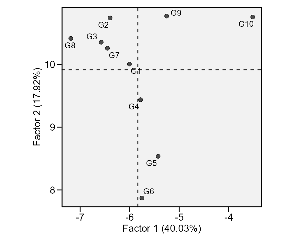
print_table(fact$GY$PCA)Wrapper function
The easiest way to compute the above-mentioned stability indexes is
by using the function ge_stats(). It is a wrapper function
that computes all the stability indexes at once. To get the results into
a “ready-to-read” file, use get_model_data().
stat_ge <- data_ge2 %>% ge_stats(ENV, GEN, REP, resp = c(EH, PH))
# Evaluating trait EH |======================                      | 50% 00:00:08
Evaluating trait PH |============================================| 100% 00:00:18
get_model_data(stat_ge, "stats") %>% print_table()
# Class of the model: ge_stats
# Variable extracted: statsIt is also possible to obtain the Spearman’s rank correlation between
the stability indexes by using corr_stab_ind().
corr_stab_ind(stat_ge)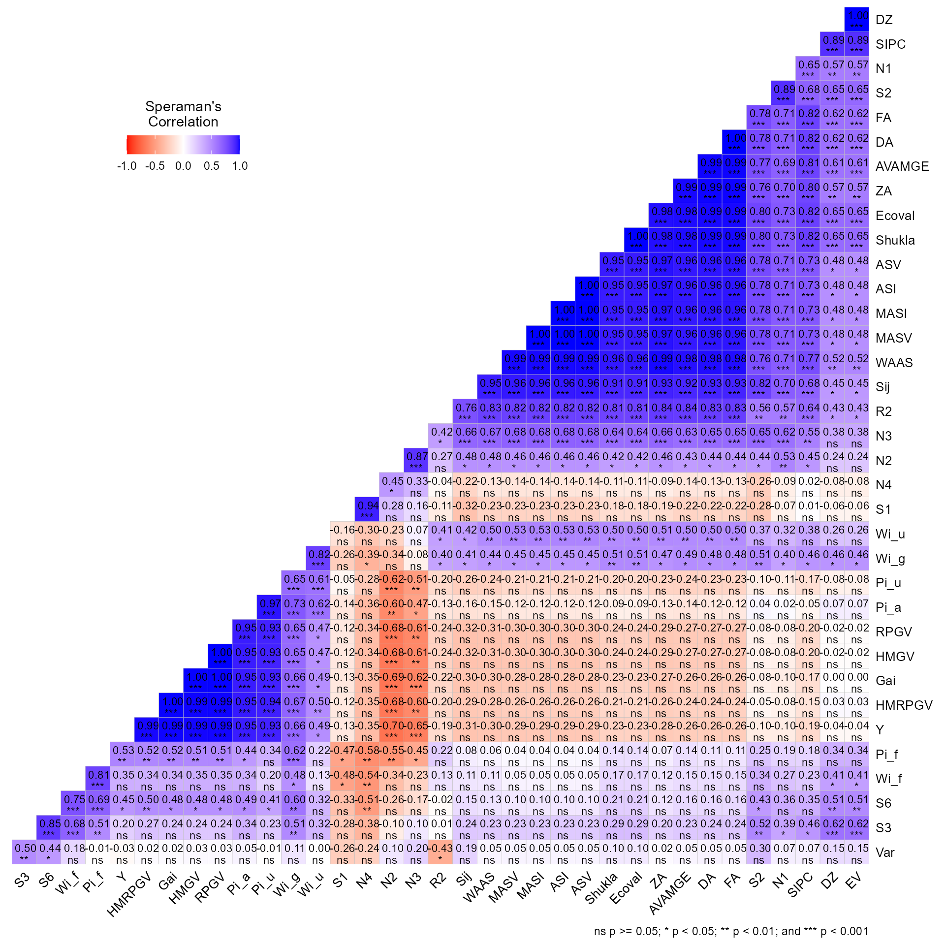
Rendering engine
This vignette was built with pkgdown. All tables were produced
with the package DT using the
following function.
library(DT) # Used to make the tables
# Function to make HTML tables
print_table <- function(table, rownames = FALSE, digits = 3, ...){
  df <- datatable(table, rownames = rownames, extensions = 'Buttons',
                  options = list(scrollX = TRUE,
                                 dom = '<<t>Bp>',
                                 buttons = c('copy', 'excel', 'pdf', 'print')), ...)
  num_cols <- c(as.numeric(which(sapply(table, class) == "numeric")))
  if(length(num_cols) > 0){
    formatSignif(df, columns = num_cols, digits = digits)
  } else{
    df
  }
}