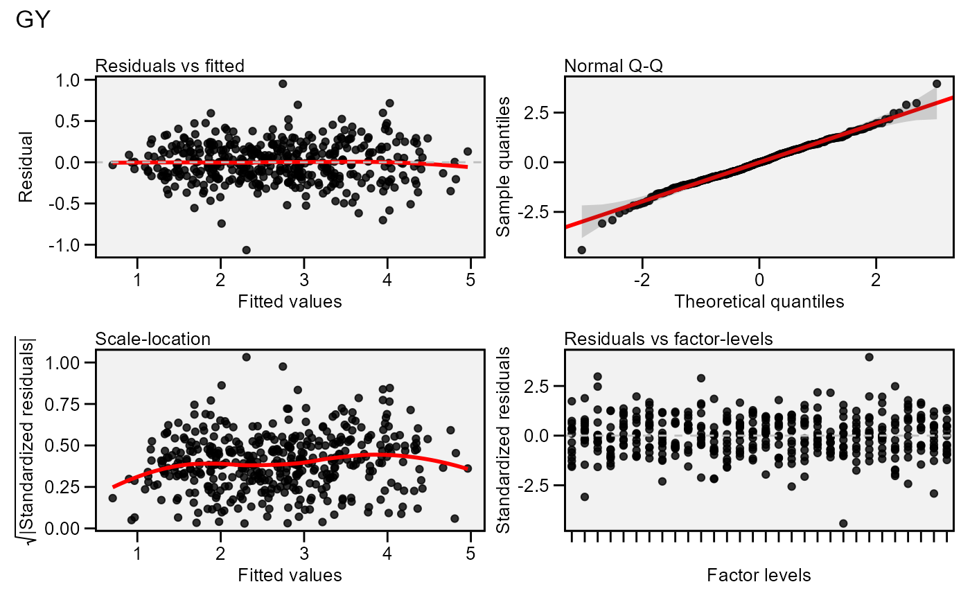
Residual plots for a output model of class anova_joint. Seven types
of plots are produced: (1) Residuals vs fitted, (2) normal Q-Q plot for the
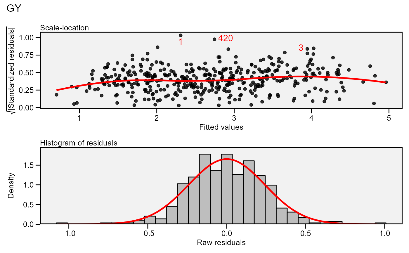
residuals, (3) scale-location plot (standardized residuals vs Fitted Values),
(4) standardized residuals vs Factor-levels, (5) Histogram of raw residuals
and (6) standardized residuals vs observation order, and (7) 1:1 line plot.
Usage
# S3 method for anova_joint
plot(x, ...)
Arguments
- x
An object of class
anova_joint.- ...
Additional arguments passed on to the function
residual_plots()
Author
Tiago Olivoto tiagoolivoto@gmail.com
Examples
# \donttest{
library(metan)
model <- anova_joint(data_ge, ENV, GEN, REP, GY)
#> variable GY
#> ---------------------------------------------------------------------------
#> Joint ANOVA table
#> ---------------------------------------------------------------------------
#> Source Df Sum Sq Mean Sq F value Pr(>F)
#> ENV 13.00 279.57 21.5057 222.41 7.25e-130
#> REP(ENV) 28.00 9.66 0.3451 3.57 3.59e-08
#> GEN 9.00 13.00 1.4439 14.93 2.19e-19
#> GEN:ENV 117.00 31.22 0.2668 2.76 1.01e-11
#> Residuals 252.00 24.37 0.0967 NA NA
#> CV(%) 11.63 NA NA NA NA
#> MSR+/MSR- 6.71 NA NA NA NA
#> OVmean 2.67 NA NA NA NA
#> ---------------------------------------------------------------------------
#>
#> All variables with significant (p < 0.05) genotype-vs-environment interaction
#> Done!
plot(model)
 plot(model,
which = c(3, 5),
nrow = 2,
labels = TRUE,
size.lab.out = 4)
#> Warning: The dot-dot notation (`..density..`) was deprecated in ggplot2 3.4.0.
#> ℹ Please use `after_stat(density)` instead.
#> ℹ The deprecated feature was likely used in the metan package.
#> Please report the issue at <https://github.com/TiagoOlivoto/metan/issues>.
plot(model,
which = c(3, 5),
nrow = 2,
labels = TRUE,
size.lab.out = 4)
#> Warning: The dot-dot notation (`..density..`) was deprecated in ggplot2 3.4.0.
#> ℹ Please use `after_stat(density)` instead.
#> ℹ The deprecated feature was likely used in the metan package.
#> Please report the issue at <https://github.com/TiagoOlivoto/metan/issues>.
 # }
# }