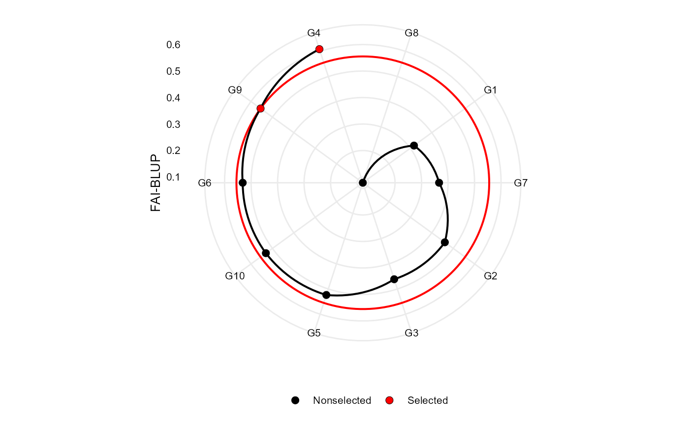
Plot the multitrait index based on factor analysis and ideotype-design proposed by Rocha et al. (2018).
Usage
# S3 method for fai_blup
plot(
  x,
  ideotype = 1,
  SI = 15,
  radar = TRUE,
  arrange.label = FALSE,
  size.point = 2.5,
  size.line = 0.7,
  size.text = 10,
  col.sel = "red",
  col.nonsel = "black",
  ...
)
Arguments
- x
An object of class
waasb- ideotype
The ideotype to be plotted. Default is 1.
- SI
An integer (0-100). The selection intensity in percentage of the total number of genotypes.
- radar
Logical argument. If true (default) a radar plot is generated after using
coord_polar().- arrange.label
Logical argument. If
TRUE, the labels are arranged to avoid text overlapping. This becomes useful when the number of genotypes is large, say, more than 30.- size.point
The size of the point in graphic. Defaults to 2.5.
- size.line
The size of the line in graphic. Defaults to 0.7.
- size.text
The size for the text in the plot. Defaults to 10.
- col.sel
The colour for selected genotypes. Defaults to
"red".- col.nonsel
The colour for nonselected genotypes. Defaults to
"black".- ...
Other arguments to be passed from ggplot2::theme().
References
Rocha, J.R.A.S.C.R, J.C. Machado, and P.C.S. Carneiro. 2018. Multitrait index based on factor analysis and ideotype-design: proposal and application on elephant grass breeding for bioenergy. GCB Bioenergy 10:52-60. doi:10.1111/gcbb.12443
Author
Tiago Olivoto tiagoolivoto@gmail.com
Examples
# \donttest{
library(metan)

mod <- waasb(data_ge,
             env = ENV,
             gen = GEN,
             rep = REP,
             resp = c(GY, HM))
#> Evaluating trait GY |======================                      | 50% 00:00:02
Evaluating trait HM |============================================| 100% 00:00:05

#> Method: REML/BLUP
#> Random effects: GEN, GEN:ENV
#> Fixed effects: ENV, REP(ENV)
#> Denominador DF: Satterthwaite's method
#> ---------------------------------------------------------------------------
#> P-values for Likelihood Ratio Test of the analyzed traits
#> ---------------------------------------------------------------------------
#>     model       GY       HM
#>  COMPLETE       NA       NA
#>       GEN 1.11e-05 5.07e-03
#>   GEN:ENV 2.15e-11 2.27e-15
#> ---------------------------------------------------------------------------
#> All variables with significant (p < 0.05) genotype-vs-environment interaction

FAI <- fai_blup(mod,
                DI = c('max, max'),
                UI = c('min, min'))
#>
#> -----------------------------------------------------------------------------------
#> Principal Component Analysis
#> -----------------------------------------------------------------------------------
#>     eigen.values cumulative.var
#> PC1          1.1          55.23
#> PC2          0.9         100.00
#>
#> -----------------------------------------------------------------------------------
#> Factor Analysis
#> -----------------------------------------------------------------------------------
#>      FA1 comunalits
#> GY -0.74       0.55
#> HM  0.74       0.55
#>
#> -----------------------------------------------------------------------------------
#> Comunalit Mean: 0.5523038
#> Selection differential
#> -----------------------------------------------------------------------------------
#>   VAR Factor        Xo        Xs          SD     SDperc    sense goal
#> 1  GY      1  2.674242  2.594199 -0.08004274 -2.9931005 increase    0
#> 2  HM      1 48.088286 48.005568 -0.08271774 -0.1720122 increase    0
#>
#> -----------------------------------------------------------------------------------
#> Selected genotypes
#> G4 G9
#> -----------------------------------------------------------------------------------
plot(FAI)

# }
# }