Plots an object of class path_coeff

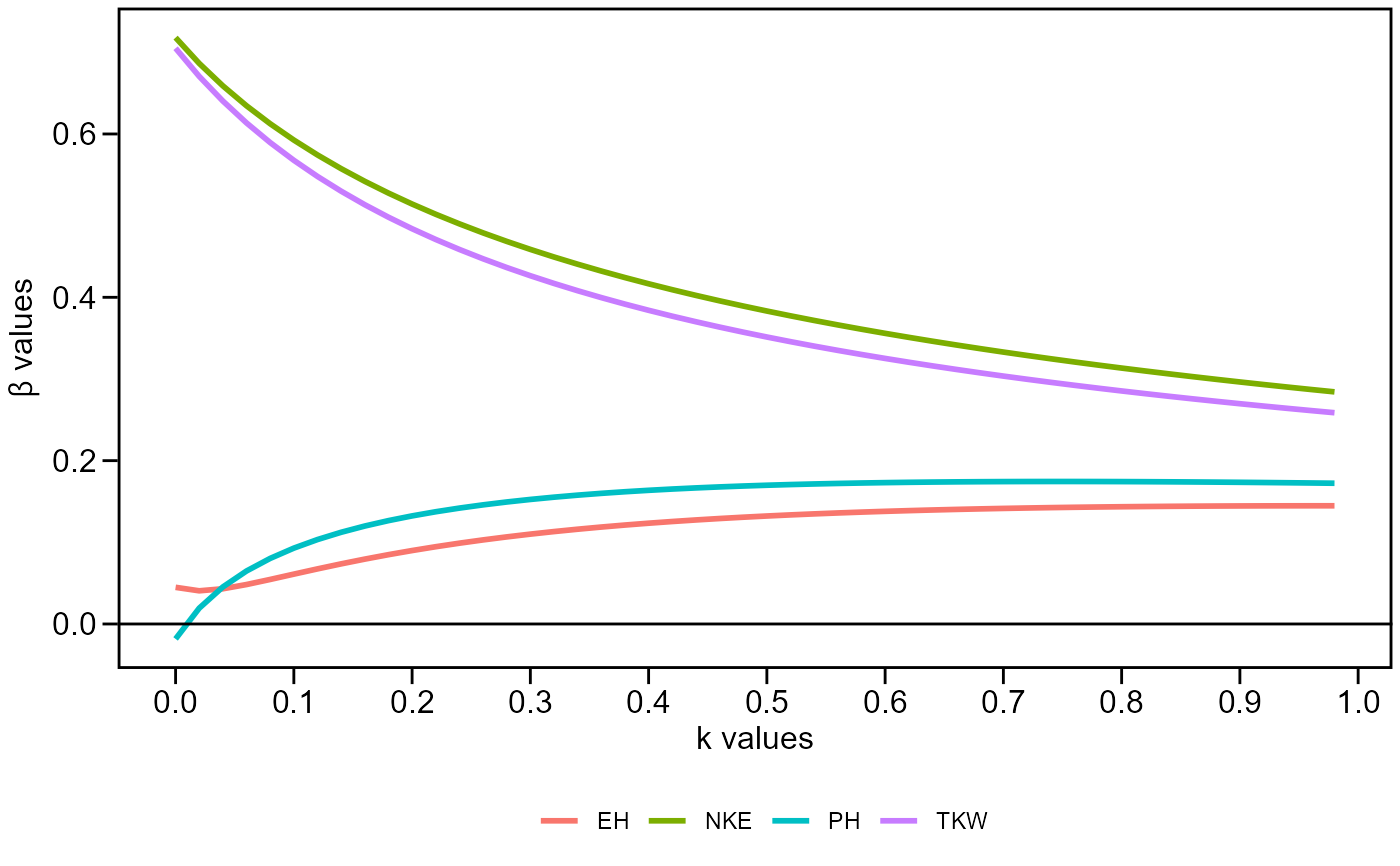
Plots an object generated by path_coeff(). Options includes the path coefficients, variance inflaction factor and the beta values with different values of 'k' values added to the diagonal of the correlation matrix of explanatory traits. See more on Details section.

Usage

# S3 method for path_coeff
plot(
  x,
  which = "coef",
  size.text.plot = 4,
  size.text.labels = 10,
  digits = 3,
  ...
)

Arguments

x

An object of class path_coeff or group_path.

which

Which to plot: one of 'coef', 'vif', or 'betas'.

size.text.plot, size.text.labels

The size of the text for plot area and labels, respectively.

digits

The significant digits to be shown.

...

Further arguments passed on to ggplot2::theme().

Details

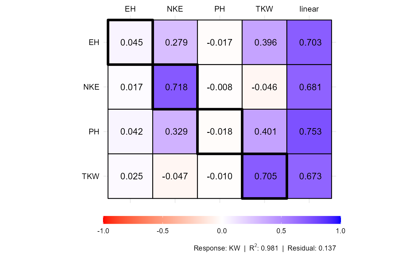
The plot which = "coef" (default) is interpreted as follows:

• The direct effects are shown in the diagonal (highlighted with a thicker line). In the example, the direct effect of NKE on KW is 0.718.

• The indirect effects are shown in the line. In the example, the indirect effect of EH on KW through TKW is 0.396.

• The linear correlation (direct + indirect) is shown in the last column.

Author

Tiago Olivoto tiagoolivoto@gmail.com

Examples

# \donttest{
library(metan)

# KW as dependent trait and all others as predictors
# PH, EH, NKE, and TKW as predictors

pcoeff <-
  path_coeff(data_ge2,
             resp = KW,
             pred = c(PH, EH, NKE, TKW))
#> Weak multicollinearity. 
#> Condition Number: 40.232
#> You will probably have path coefficients close to being unbiased. 
plot(pcoeff)

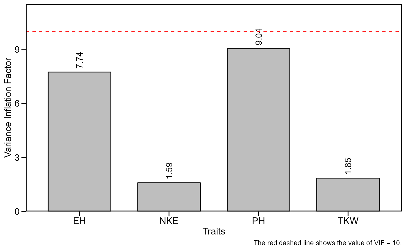
plot(pcoeff, which = "vif")

plot(pcoeff, which = "betas")

# }