![[Stable]](figures/lifecycle-stable.svg)
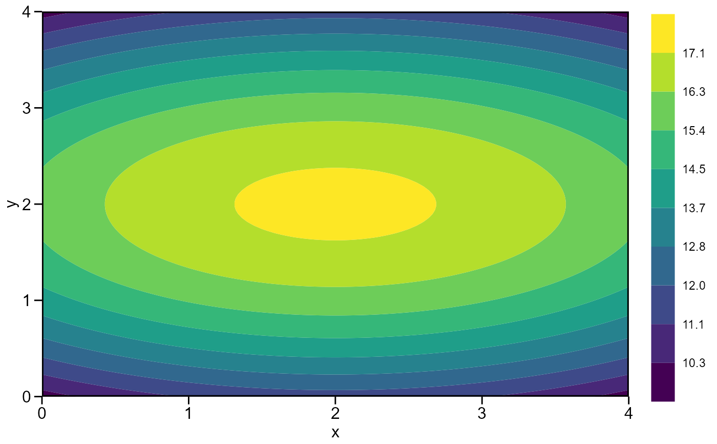
Compute a surface model and find the best combination of factor1 and factor2 to obtain the stationary point.
Arguments
- .data
The dataset containing the columns related to Environments, factor1, factor2, replication/block and response variable(s).
- factor1
The first factor, for example, dose of Nitrogen.
- factor2
The second factor, for example, dose of potassium.
- rep
The name of the column that contains the levels of the replications/blocks, if a designed experiment was conducted. Defaults to
NULL.- resp
The response variable(s).
- prob
The probability error.
- verbose
If
verbose = TRUEthen some results are shown in the console.
Author
Tiago Olivoto tiagoolivoto@gmail.com
Examples
# \donttest{
library(metan)
# A small toy example

df <- data.frame(
 expand.grid(x = seq(0, 4, by = 1),
             y = seq(0, 4, by = 1)),
 z = c(10, 11, 12, 11, 10,
       14, 15, 16, 15, 14,
       16, 17, 18, 17, 16,
       14, 15, 16, 15, 14,
       10, 11, 12, 11, 10)
)
mod <- resp_surf(df, x, y, resp = z)
#> -----------------------------------------------------------------
#> Anova table for the response surface model
#> -----------------------------------------------------------------
#> Analysis of Variance Table
#>
#> Response: z
#>           Df  Sum Sq Mean Sq F value    Pr(>F)
#> x          1   0.000   0.000    0.00         1
#> y          1   0.000   0.000    0.00         1
#> I(x^2)     1  12.857  12.857  106.88 3.073e-09 ***
#> I(y^2)     1 142.857 142.857 1187.50 < 2.2e-16 ***
#> x:y        1   0.000   0.000    0.00         1
#> Residuals 19   2.286   0.120
#> ---
#> Signif. codes:  0 '***' 0.001 '**' 0.01 '*' 0.05 '.' 0.1 ' ' 1
#> -----------------------------------------------------------------
#> Model equation for response surface model
#> Y = B0 + B1*A + B2*D + B3*A^2 + B4*D^2 + B5*A*D
#> -----------------------------------------------------------------
#> Estimated parameters
#> B0: 9.8857143
#> B1: 1.7142857
#> B2: 5.7142857
#> B3: -0.4285714
#> B4: -1.4285714
#> B5: 0.0000000
#> -----------------------------------------------------------------
#> Matrix of parameters (A)
#> -----------------------------------------------------------------
#> -0.4285714    0.0000000
#> 0.0000000    -1.4285714
#> -----------------------------------------------------------------
#> Inverse of the matrix A (invA)
#> -2.3333333    0.0000000
#> 0.0000000    -0.7000000
#> -----------------------------------------------------------------
#> Vetor of parameters B1 e B2 (X)
#> -----------------------------------------------------------------
#> B1: 1.7142857
#> B2: 5.7142857
#> -----------------------------------------------------------------
#> Equation for the optimal points (A and D)
#> -----------------------------------------------------------------
#> -0.5*(invA*X)
#> Eigenvalue 1: -0.428571
#> Eigenvalue 2: -1.428571
#> Stacionary point is maximum!
#> -----------------------------------------------------------------
#> Stacionary point obtained with the following original units:
#> -----------------------------------------------------------------
#> Optimal dose (x): 2
#> Optimal dose (y): 2
#> Predicted: 17.3143
#> -----------------------------------------------------------------
#> Fitted model
#> -----------------------------------------------------------------
#> A = x
#> D = y
#> y = 9.88571+1.71429A+5.71429D+-0.42857A^2+-1.42857D^2+0A*D
#> -----------------------------------------------------------------
#> Shapiro-Wilk normality test
#> p-value:  0.04213785
#> WARNING: at 5% of significance, residuals can not be considered normal!
#> ------------------------------------------------------------------
plot(mod)

# }
# }