If more than one index is available, the function performs a Principal
Component Analysis and produces a plot showing the contribution of the
indexes to the PC1 (see pca()). If an index is declared in
index and a cut point in cut_point, the number and proportion of objects
with mean value of index bellow and above cut_point are returned.
Additionaly, the number and proportion of pixels bellow and above the
cutpoint is shown for each object (id).
Usage
summary_index(
  object,
  index = NULL,
  cut_point = NULL,
  select_higher = FALSE,
  plot = TRUE,
  type = "var",
  ...
)
Arguments
- object
An object computed with
analyze_objects().- index
The index desired, e.g.,
"B". Note that these value must match the index(es) used in the argumentobject_indexofanalyze_objects().- cut_point
The cut point.
- select_higher
If
FALSE(default) selects the objects withindexsmaller than thecut_point. Useselect_higher = TRUEto select the objects withindexhigher thancut_point.- plot
Shows the contribution plot when more than one index is available? Defaults to
TRUE.- type
The type of plot to produce. Defaults to
"var". See more atget_biplot().- ...
Further arguments passed on to
get_biplot().
Value
A list with the following elements:
idsThe identification of selected objects.between_idA data frame with the following columnsnThe number of objects.nselThe number of selected objects.propThe proportion of objects selected.mean_index_sel, andmean_index_nselThe mean value ofindexfor the selected and non-selected objects, respectively.
within_idA data frame with the following columnsidThe object identificationn_lessThe number of pixels with values lesser than or equal tocut_point.n_greaterThe number of pixels with values greater thancut_point.less_ratioThe proportion of pixels with values lesser than or equal tocut_point.greater_ratioThe proportion of pixels with values greater thancut_point.
pca_resAn object computed withpca()
Author
Tiago Olivoto tiagoolivoto@gmail.com
Examples
library(pliman)
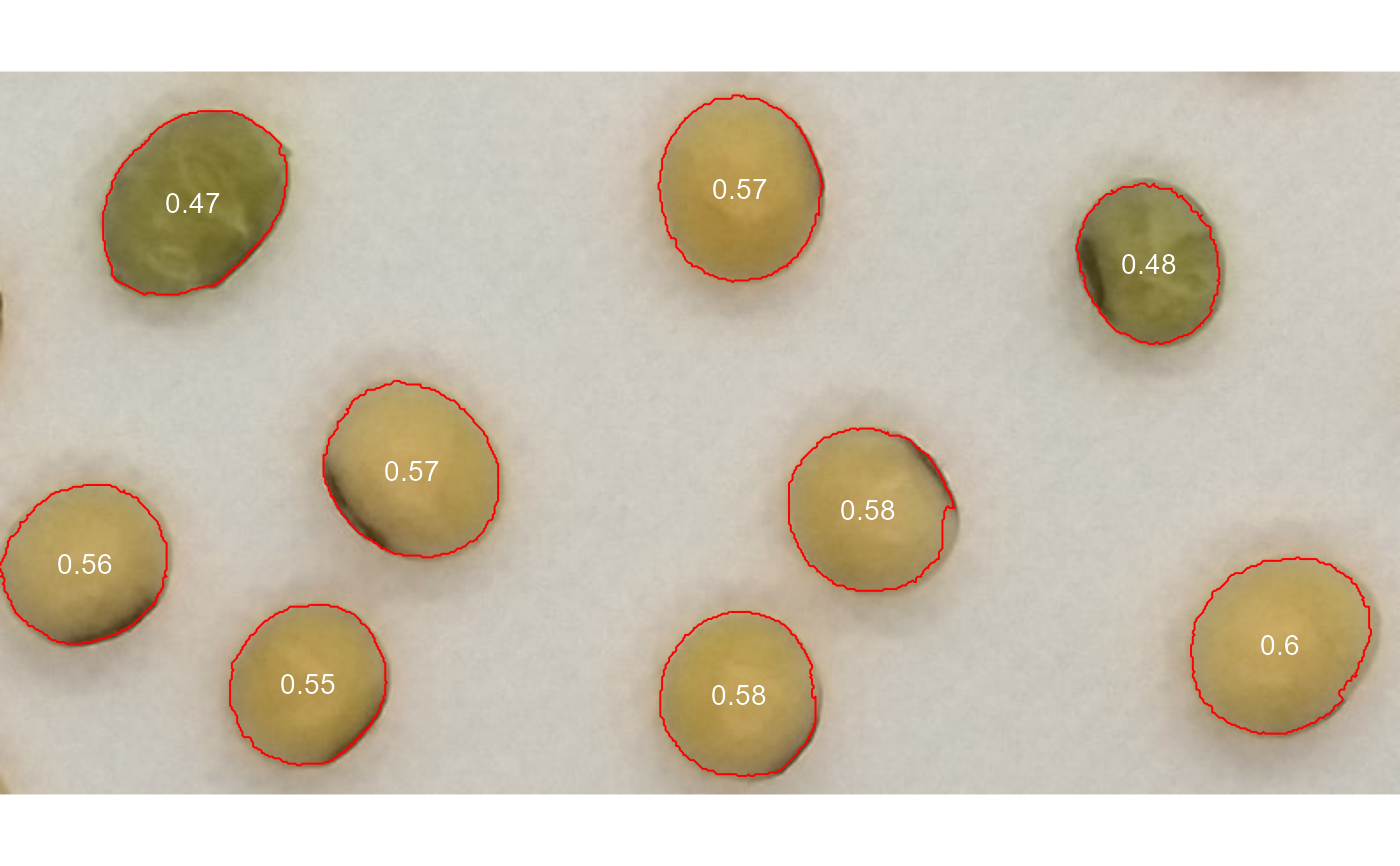
soy <- image_pliman("soy_green.jpg")
anal <- analyze_objects(soy, object_index = "G", pixel_level_index = TRUE)
plot_measures(anal, measure = "G")


summary_index(anal, index = "G", cut_point = 0.5)
