01: Desempenho agronômico do linho em diferentes épocas de semeadura
1 Pacotes
To reproduce the examples of this material, the R packages the following packages are needed.
2 Dados
df_p <-
  import("data/data_parcelas.csv")
3 Análise de variância
3.1 Rendimento de grãos
modrg <- with(df_p,
            PSUBDBC(epoca, cultivar, bloco, rgha,
                    xlab = "Épocas de semeadura"))
##
## -----------------------------------------------------------------
## Normality of errors
## -----------------------------------------------------------------
##                          Method Statistic    p.value
##  Shapiro-Wilk normality test(W) 0.8962594 0.01794671
##
##
##
## -----------------------------------------------------------------
## Homogeneity of Variances
## -----------------------------------------------------------------
## Plot
##                               Method Statistic      p.value
##  Bartlett test(Bartlett's K-squared)  27.67379 4.252128e-06
##
##
## ----------------------------------------------------
## Split-plot
##                               Method Statistic   p.value
##  Bartlett test(Bartlett's K-squared)  2.030255 0.1541947
##
##
## ----------------------------------------------------
## Interaction
##                               Method Statistic     p.value
##  Bartlett test(Bartlett's K-squared)  23.33425 0.001490467
##
##
## -----------------------------------------------------------------
## Additional Information
## -----------------------------------------------------------------
##
## CV1 (%) =  14.97
## CV2 (%) =  34.61
## Mean =  743.825
## Median =  533.9
##
## -----------------------------------------------------------------
## Analysis of Variance
## -----------------------------------------------------------------
##         Df Sum Sq      Mean Sq     F value     Pr(>F)
## F1      3  6881050.432 2293683.477 185.0987045 p<0.001
## Block   2     2873.868    1436.934   0.1159596 0.892
## Error A 6    74350.066   12391.678
## F2      1     4298.727    4298.727   0.0648632 0.805
## F1 x F2 3   105689.020   35229.673   0.5315782 0.673
## Error B 8   530189.913   66273.739
## -----------------------------------------------------------------
## No significant interaction
## -----------------------------------------------------------------
##
## -----------------------------------------------------------------
## F1
## -----------------------------------------------------------------
## Multiple Comparison Test: Tukey HSD
##         resp groups
## E1 1469.8333      a
## E2 1045.8667      b
## E4  236.1667      c
## E3  223.4333      c
##
##
## -----------------------------------------------------------------
## Isolated factors 2 not significant
## -----------------------------------------------------------------
##       Mean
## D 730.4417
## M 757.2083

rg <-
modrg$graph1 +
  labs(x = "Épocas de semeadura",
       y = expression(Rendimento~de~grãos~(kg~ha^{-1})))
3.2 Massa de mil grãos
modmmg <- with(df_p,
            PSUBDBC(epoca, cultivar, bloco, mmg))
##
## -----------------------------------------------------------------
## Normality of errors
## -----------------------------------------------------------------
##                          Method Statistic   p.value
##  Shapiro-Wilk normality test(W) 0.9587968 0.4147291
##
##
##
## -----------------------------------------------------------------
## Homogeneity of Variances
## -----------------------------------------------------------------
## Plot
##                               Method Statistic   p.value
##  Bartlett test(Bartlett's K-squared)  1.522785 0.6770217
##
##
## ----------------------------------------------------
## Split-plot
##                               Method Statistic   p.value
##  Bartlett test(Bartlett's K-squared) 0.3166758 0.5736123
##
##
## ----------------------------------------------------
## Interaction
##                               Method Statistic   p.value
##  Bartlett test(Bartlett's K-squared)  7.564106 0.3725931
##
##
## -----------------------------------------------------------------
## Additional Information
## -----------------------------------------------------------------
##
## CV1 (%) =  17.2
## CV2 (%) =  11.93
## Mean =  4.8387
## Median =  4.9463
##
## -----------------------------------------------------------------
## Analysis of Variance
## -----------------------------------------------------------------
##         Df     Sum Sq   Mean Sq    F value Pr(>F)
## F1       3 22.2493125 7.4164375 10.7060422  0.008
## Block    2  0.6355228 0.3177614  0.4587063  0.653
## Error A  6  4.1564029 0.6927338
## F2       1  0.9561335 0.9561335  2.8715898  0.129
## F1 x F2  3  2.3794528 0.7931509  2.3820984  0.145
## Error B  8  2.6637050 0.3329631
## -----------------------------------------------------------------
## No significant interaction
## -----------------------------------------------------------------
##
## -----------------------------------------------------------------
## F1
## -----------------------------------------------------------------
## Multiple Comparison Test: Tukey HSD
##        resp groups
## E2 5.857779      a
## E1 5.743322      a
## E4 3.898390      b
## E3 3.855251      b
##
##
## -----------------------------------------------------------------
## Isolated factors 2 not significant
## -----------------------------------------------------------------
##       Mean
## D 5.038282
## M 4.639089
mmg <-
  modmmg$graph1 +
  labs(x = "Épocas de semeadura",
       y = "Massa de mil grãos (g)")

arrange_ggplot(rg, mmg,
               tag_levels = "a")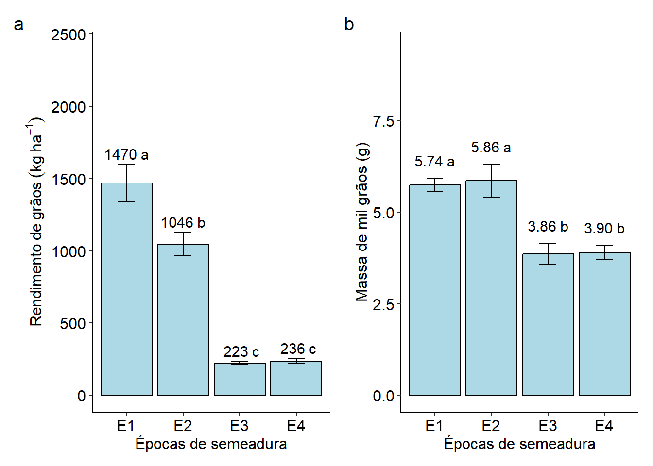
ggsave("figs/rg_mmg.jpg",
       width = 8,
       height = 4)
3.3 Número de cápsulas
modnc <- with(df_p,
            PSUBDBC(epoca, cultivar, bloco, nc))
##
## -----------------------------------------------------------------
## Normality of errors
## -----------------------------------------------------------------
##                          Method Statistic   p.value
##  Shapiro-Wilk normality test(W) 0.9498939 0.2695177
##
##
##
## -----------------------------------------------------------------
## Homogeneity of Variances
## -----------------------------------------------------------------
## Plot
##                               Method Statistic   p.value
##  Bartlett test(Bartlett's K-squared)  1.510963 0.6797424
##
##
## ----------------------------------------------------
## Split-plot
##                               Method Statistic   p.value
##  Bartlett test(Bartlett's K-squared) 0.0277831 0.8676198
##
##
## ----------------------------------------------------
## Interaction
##                               Method Statistic   p.value
##  Bartlett test(Bartlett's K-squared)  2.553598 0.9230073
##
##
## -----------------------------------------------------------------
## Additional Information
## -----------------------------------------------------------------
##
## CV1 (%) =  32.15
## CV2 (%) =  9.72
## Mean =  21.7385
## Median =  21
##
## -----------------------------------------------------------------
## Analysis of Variance
## -----------------------------------------------------------------
##         Df     Sum Sq   Mean Sq    F value Pr(>F)
## F1       3 1076.18417 358.72806  7.3462116  0.020
## Block    2   38.21202  19.10601  0.3912624  0.692
## Error A  6  292.99025  48.83171
## F2       1   66.32847  66.32847 14.8571981  0.005
## F1 x F2  3   45.72412  15.24137  3.4139807  0.073
## Error B  8   35.71520   4.46440
## -----------------------------------------------------------------
## No significant interaction
## -----------------------------------------------------------------
##
## -----------------------------------------------------------------
## F1
## -----------------------------------------------------------------
## Multiple Comparison Test: Tukey HSD
##        resp groups
## E1 31.99954      a
## E2 23.40231     ab
## E3 16.09656      b
## E4 15.45556      b
##
##
##
## -----------------------------------------------------------------
## F2
## -----------------------------------------------------------------
## Multiple Comparison Test: Tukey HSD
##       resp groups
## D 23.40093      a
## M 20.07606      b
pnce <-
  modnc$graph1 +
  labs(x = "Épocas de semeadura",
       y = "Número de cápsulas")

pncc <-
  modnc$graph2 +
  labs(x = "Cultivares",
       y = "Número de cápsulas")

arrange_ggplot(pnce, pncc, widths = c(0.75, 0.25), tag_levels = "a")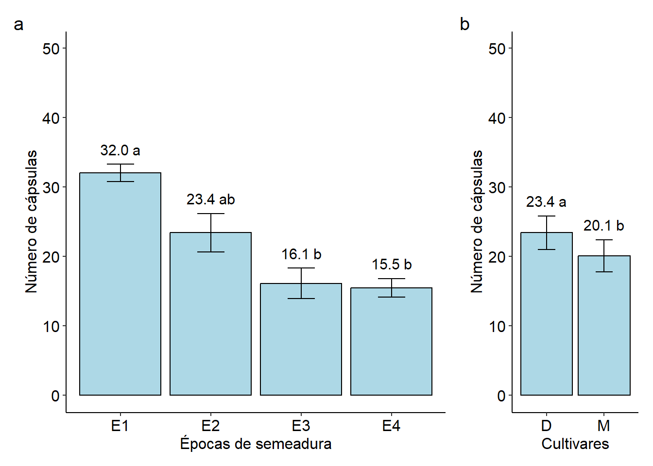
ggsave("figs/nc.jpg",
       width = 8,
       height = 4)
4 Correlação
corr_coef(df_p, rgha, mmg, nc) |>
  network_plot(legend_position = "bottom")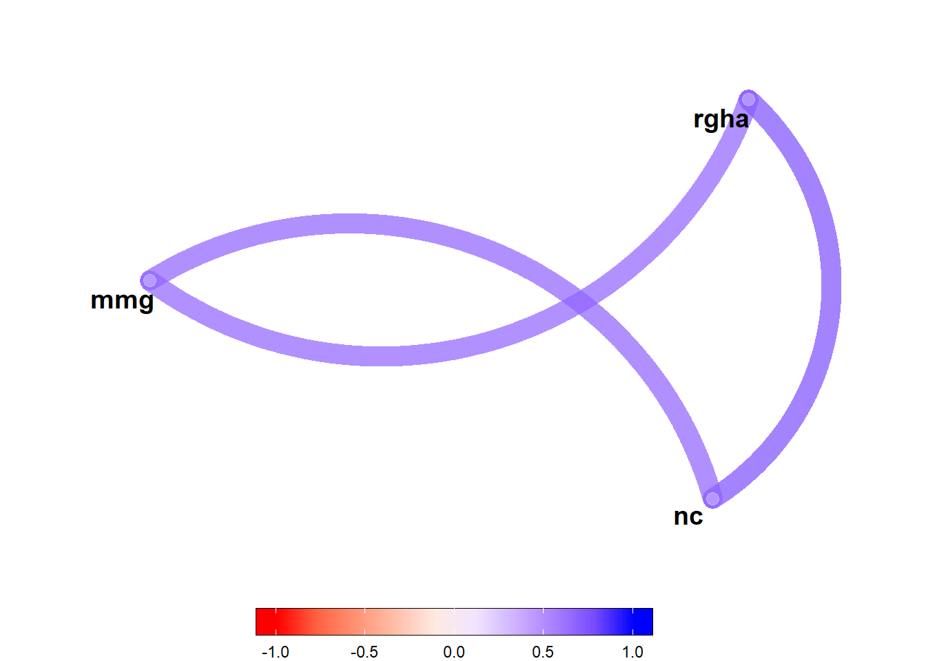
ggsave("figs/corr_epocas.jpg",
       width = 10,
       height = 3)
5 Section info
sessionInfo()
## R version 4.2.2 (2022-10-31 ucrt)
## Platform: x86_64-w64-mingw32/x64 (64-bit)
## Running under: Windows 10 x64 (build 22621)
##
## Matrix products: default
##
## locale:
## [1] LC_COLLATE=Portuguese_Brazil.utf8  LC_CTYPE=Portuguese_Brazil.utf8
## [3] LC_MONETARY=Portuguese_Brazil.utf8 LC_NUMERIC=C
## [5] LC_TIME=Portuguese_Brazil.utf8
##
## attached base packages:
## [1] stats     graphics  grDevices utils     datasets  methods   base
##
## other attached packages:
##  [1] metan_1.18.0    AgroR_1.3.3     lubridate_1.9.2 forcats_1.0.0
##  [5] stringr_1.5.0   dplyr_1.1.2     purrr_1.0.1     readr_2.1.4
##  [9] tidyr_1.3.0     tibble_3.2.1    ggplot2_3.4.2   tidyverse_2.0.0
## [13] rio_0.5.29
##
## loaded via a namespace (and not attached):
##  [1] nlme_3.1-160        RColorBrewer_1.1-3  numDeriv_2016.8-1.1
##  [4] tools_4.2.2         utf8_1.2.3          R6_2.5.1
##  [7] nortest_1.0-4       colorspace_2.1-0    withr_2.5.0
## [10] GGally_2.1.2        tidyselect_1.2.0    gridExtra_2.3
## [13] emmeans_1.8.7       curl_5.0.1          compiler_4.2.2
## [16] textshaping_0.3.6   cli_3.6.1           sandwich_3.0-2
## [19] labeling_0.4.2      scales_1.2.1        lmtest_0.9-40
## [22] mvtnorm_1.2-2       multcompView_0.1-9  systemfonts_1.0.4
## [25] digest_0.6.33       foreign_0.8-83      minqa_1.2.5
## [28] rmarkdown_2.23      pkgconfig_2.0.3     htmltools_0.5.5
## [31] lme4_1.1-34         plotrix_3.8-2       fastmap_1.1.1
## [34] dunn.test_1.3.5     htmlwidgets_1.6.2   rlang_1.1.1
## [37] readxl_1.4.3        rstudioapi_0.15.0   farver_2.1.1
## [40] generics_0.1.3      zoo_1.8-12          jsonlite_1.8.7
## [43] gtools_3.9.4        zip_2.3.0           car_3.1-2
## [46] magrittr_2.0.3      patchwork_1.1.2     Matrix_1.6-0
## [49] Rcpp_1.0.11         munsell_0.5.0       fansi_1.0.4
## [52] abind_1.4-5         lifecycle_1.0.3     stringi_1.7.12
## [55] multcomp_1.4-25     yaml_2.3.7          carData_3.0-5
## [58] mathjaxr_1.6-0      MASS_7.3-60         plyr_1.8.8
## [61] grid_4.2.2          ggrepel_0.9.3       crayon_1.5.2
## [64] lattice_0.20-45     haven_2.5.3         cowplot_1.1.1
## [67] splines_4.2.2       hms_1.1.3           knitr_1.43
## [70] pillar_1.9.0        boot_1.3-28         estimability_1.4.1
## [73] codetools_0.2-18    glue_1.6.2          drc_3.0-1
## [76] evaluate_0.21       data.table_1.14.8   tweenr_2.0.2
## [79] vctrs_0.6.3         nloptr_2.0.3        tzdb_0.4.0
## [82] cellranger_1.1.0    polyclip_1.10-4     gtable_0.3.3
## [85] reshape_0.8.9       ggforce_0.4.1       xfun_0.39
## [88] openxlsx_4.2.5.2    xtable_1.8-4        coda_0.19-4
## [91] ragg_1.2.5          survival_3.4-0      lmerTest_3.1-3
## [94] timechange_0.2.0    TH.data_1.1-2