library(rio)
library(tidyverse)
library(metan)

gdi <- function(dfrc,
                gen,
                vars =  NULL,
                si = 0.2,
                ideotype = NULL){

  if(missing(vars)){
    gen <-  dfrc |> select({{gen}})
    vars <- dfrc |> select_numeric_cols()
    dfrc <- bind_cols(gen, vars)
  } else{
    gen <-  dfrc |> select({{gen}})
    vars <- dfrc |> select({{vars}})
    dfrc <- bind_cols(gen, vars)
  }

  mger <- dfrc |> mean_by()
  dfrc_num <- dfrc |> select_numeric_cols()
  nvars <- ncol(dfrc_num)
  ngen <- nrow(dfrc_num)

  varn <- colnames(dfrc_num)

  ifelse(is.null(ideotype),
         ideotype <- rep("h", nvars),
         ideotype <- ideotype)

  results <- data.frame(matrix(NA, nvars, nvars))
  results_perc <- data.frame(matrix(NA, nvars, nvars))
  ngensel <- ceiling(ngen * si)
  selgen <- list()

  # selecao direta e indireta
  for (i  in 1:nvars){
    if(ideotype[i] == "h"){
      msel <-
        dfrc |>
        slice_max(dfrc_num[, i], n = ngensel)

      selgen[[i]] <- msel |> pull(1)
      msel <- msel |>  mean_by()
      results[i, ] <- msel - mger
      results_perc[i, ] <- (msel - mger) / mger * 100
    } else{
      msel <-
        dfrc |>
        slice_min(dfrc_num[, i], n = ngensel) |>
        mean_by()

      selgen[[i]] <- msel |> pull(1)

      msel <- msel |>  mean_by()

      results[i, ] <- msel - mger
      results_perc[i, ] <- (msel - mger) / mger * 100

    }
  }
  colnames(results) <- rownames(results) <- varn
  colnames(results_perc) <- rownames(results_perc) <-  varn
  print(selgen)
  names(selgen) <- varn

  return(list(results = results,
              results_perc = results_perc,
              selgen = selgen))
}


######## plotar os valores
plot_gdi <- function(model,
                     type = c("percent", "absolut"),
                     range_scale = NULL){
  type <- type[1]

  if(type == "percent"){
    df_plot <-
      model$results_perc |>
      make_long()

  } else{
    df_plot <-
      model$results |>
      make_long()
  }


  fcts <- as.character(unique(factor(df_plot$ENV)))
  df_plot <-
    df_plot %>%
    mutate(lwid = ifelse((ENV == GEN), 1.5, 0.5)) %>%
    mutate(ENV =  factor(as.factor(ENV), levels = c(fcts, "linear"))) %>%
    mutate(GEN = factor(as.factor(GEN), levels = rev(fcts))) %>%
    arrange(lwid)


  ifelse(is.null(range_scale),
         rang <- range(df_plot$Y),
         rang <- range_scale)
  ggplot(df_plot, aes(ENV, GEN, fill = Y)) +
    geom_tile(color = "black",
              linewidth = df_plot$lwid) +
    scale_fill_gradient2(low = "red",
                         high = "blue",
                         mid = "white",
                         midpoint = mean(df_plot$Y),
                         limit = rang,
                         space = "Lab",
                         na.value = "transparent") +
    geom_text(aes(label = round(Y, 1)),
              color = "black",
              size = 3) +
    guides(fill = guide_colourbar(label = TRUE,
                                  draw.ulim = TRUE,
                                  draw.llim = TRUE,
                                  frame.colour = "black",
                                  ticks = TRUE,
                                  nbin = 10,
                                  label.position = "right",
                                  barwidth = 1,
                                  barheight = 11,
                                  direction = 'vertical')) +
    scale_y_discrete(expand = expansion(mult = c(0,0))) +
    scale_x_discrete(position = "top",
                     expand = expansion(0)) +
    labs(x = NULL,
         y = NULL,
         fill = "SD (%)")
}02: Diferencial de seleção direto e indireto visando seleção de genótipos de linho
1 Pacotes
2 Dados
df <-
  import("data/data_mgidi.csv") |>
  remove_rows_na() |>
  filter(epoca %in% c("E1", "E4")) |>
  replace_string(epoca, pattern = "E4", replacement = "E2")

# por época
dfe <-
  df |>
  split_factors(epoca)
3 Correlação parcial
# correlação parcial
res_part <- lapply(dfe, corr_coef)
p1 <- network_plot(res_part$E1)
p2 <- network_plot(res_part$E2)
arrange_ggplot(p1, p2)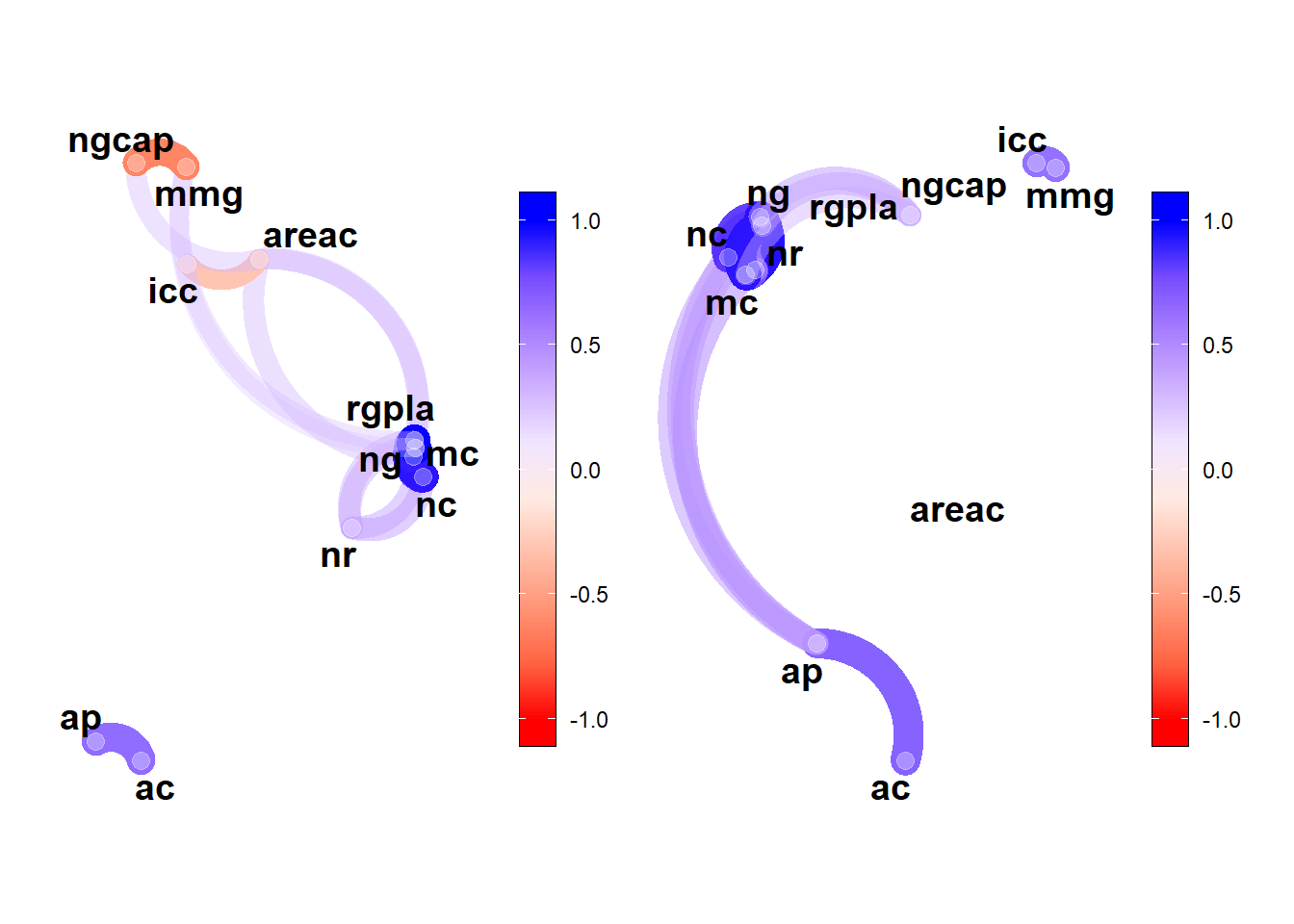
ggsave("figs/corr_linear.jpg",
       width = 10,
       height = 6)
4 Histogram
library(ggridges)

ggplot(df, aes(rgpla, y = epoca)) +
  geom_density_ridges(aes(fill = epoca),
                      scale = 3) +
  theme_bw() +
  scale_y_discrete(expand = expansion(c(0.2, 0.2))) +
  theme_bw(base_size = 18) +
  theme()+
  labs(fill = "",
       x = "Rendimento de grãos por planta (g)",
       y = "Época de semeadura")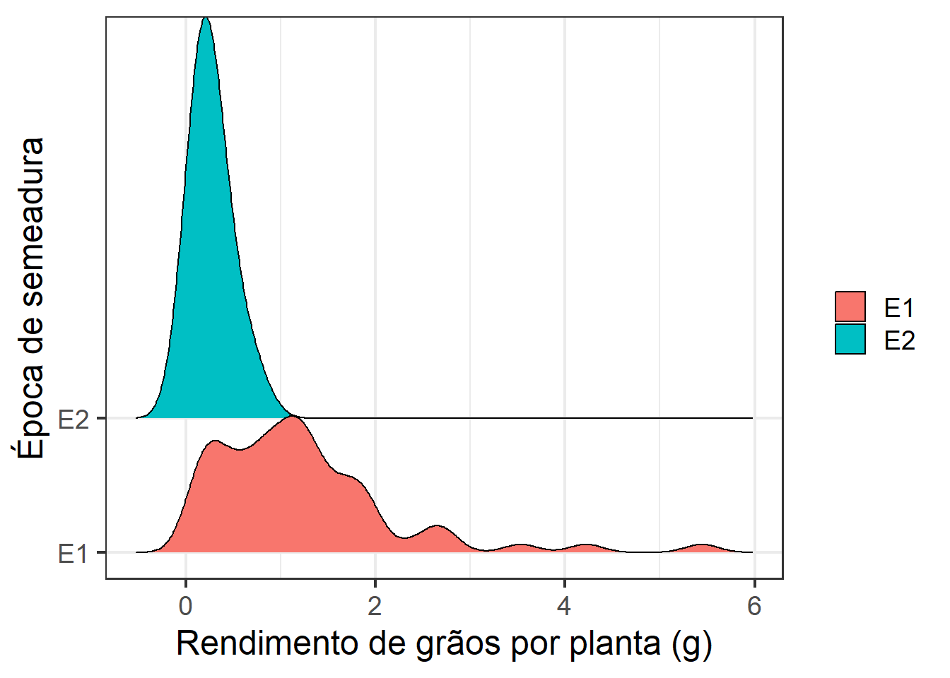
ggsave("figs/density_gy.jpg",
       width = 6,
       height = 4)
5 Diferencial de seleção
# diferencial de seleção por época
res_epoca <- lapply(dfe, gdi, gen,
                    si = 0.25,
                    ideotype = c("l", rep("h", 10)))
## [[1]]
## [1] 67.52632
##
## [[2]]
##  [1] "G46" "G44" "G30" "G9"  "G26" "G49" "G10" "G17" "G27" "G34" "G35" "G48"
## [13] "G32" "G14" "G4"  "G41" "G51"
##
## [[3]]
##  [1] "G228" "G4"   "G48"  "G13"  "G36"  "G233" "G29"  "G41"  "G230" "G222"
## [11] "G216" "G9"   "G28"  "G31"  "G3"   "G226" "G19"  "G20"  "G33"
##
## [[4]]
##  [1] "G228" "G4"   "G48"  "G13"  "G233" "G36"  "G31"  "G222" "G41"  "G230"
## [11] "G29"  "G3"   "G9"   "G33"  "G223" "G216" "G14"
##
## [[5]]
##  [1] "G222" "G31"  "G228" "G219" "G30"  "G9"   "G10"  "G17"  "G15"  "G5"
## [11] "G45"  "G223" "G28"  "G235" "G8"   "G47"  "G224"
##
## [[6]]
##  [1] "G230" "G29"  "G38"  "G41"  "G47"  "G215" "G219" "G222" "G228" "G232"
## [11] "G233" "G10"  "G13"  "G14"  "G16"  "G19"  "G20"  "G27"  "G33"  "G35"
## [21] "G36"  "G40"  "G49"  "G216" "G218" "G225" "G226" "G235"
##
## [[7]]
##  [1] "G228" "G4"   "G48"  "G13"  "G36"  "G222" "G29"  "G41"  "G230" "G233"
## [11] "G216" "G9"   "G28"  "G3"   "G31"  "G10"  "G20"
##
## [[8]]
##  [1] "G228" "G4"   "G48"  "G13"  "G36"  "G222" "G29"  "G9"   "G233" "G41"
## [11] "G28"  "G3"   "G216" "G31"  "G230" "G20"  "G215"
##
## [[9]]
##  [1] "G234" "G27"  "G22"  "G44"  "G5"   "G9"   "G215" "G20"  "G46"  "G232"
## [11] "G29"  "G19"  "G39"  "G40"  "G16"  "G3"   "G1"
##
## [[10]]
##  [1] "G35"  "G31"  "G235" "G5"   "G2"   "G229" "G225" "G228" "G224" "G222"
## [11] "G234" "G223" "G3"   "G39"  "G33"  "G40"  "G44"
##
## [[11]]
##  [1] "G28"  "G27"  "G50"  "G21"  "G20"  "G29"  "G30"  "G215" "G19"  "G48"
## [11] "G22"  "G9"   "G23"  "G216" "G222" "G46"  "G10"
##
## [[1]]
## [1] 60.53333
##
## [[2]]
##  [1] "G193" "G170" "G160" "G166" "G169" "G181" "G167" "G161" "G178" "G180"
## [11] "G183" "G207" "G164" "G201"
##
## [[3]]
##  [1] "G205" "G177" "G206" "G161" "G195" "G196" "G170" "G188" "G201" "G197"
## [11] "G175" "G167" "G200" "G203" "G211"
##
## [[4]]
##  [1] "G177" "G206" "G170" "G195" "G205" "G161" "G200" "G197" "G196" "G203"
## [11] "G175" "G163" "G174" "G201"
##
## [[5]]
##  [1] "G165" "G167" "G192" "G160" "G169" "G168" "G200" "G191" "G190" "G195"
## [11] "G161" "G179" "G188" "G163"
##
## [[6]]
##  [1] "G205" "G162" "G163" "G177" "G188" "G196" "G197" "G206" "G161" "G164"
## [11] "G175" "G185" "G190" "G160" "G165" "G166" "G167" "G168" "G169" "G170"
## [21] "G171" "G172" "G173" "G174" "G176" "G178" "G179" "G180" "G181" "G182"
## [31] "G183" "G184" "G186" "G187" "G189" "G191" "G192" "G193" "G194" "G195"
## [41] "G198" "G199" "G200" "G201" "G202" "G203" "G204" "G207" "G208" "G209"
## [51] "G210" "G211" "G212" "G213" "G214"
##
## [[7]]
##  [1] "G177" "G206" "G170" "G195" "G205" "G161" "G196" "G197" "G200" "G167"
## [11] "G203" "G163" "G201" "G188"
##
## [[8]]
##  [1] "G177" "G195" "G161" "G206" "G170" "G205" "G197" "G200" "G196" "G203"
## [11] "G163" "G167" "G160" "G169" "G174"
##
## [[9]]
##  [1] "G189" "G161" "G192" "G202" "G185" "G180" "G174" "G183" "G200" "G191"
## [11] "G197" "G195" "G178" "G210"
##
## [[10]]
##  [1] "G192" "G170" "G204" "G200" "G195" "G194" "G163" "G184" "G214" "G168"
## [11] "G197" "G183" "G203" "G177"
##
## [[11]]
##  [1] "G189" "G210" "G180" "G165" "G202" "G160" "G196" "G161" "G197" "G185"
## [11] "G191" "G167" "G195" "G188"
g1 <- plot_gdi(res_epoca$E1, range_scale = c(-70, 195))
g2 <- plot_gdi(res_epoca$E2, range_scale = c(-70, 195))
arrange_ggplot(g1, g2,
               tag_levels = "a")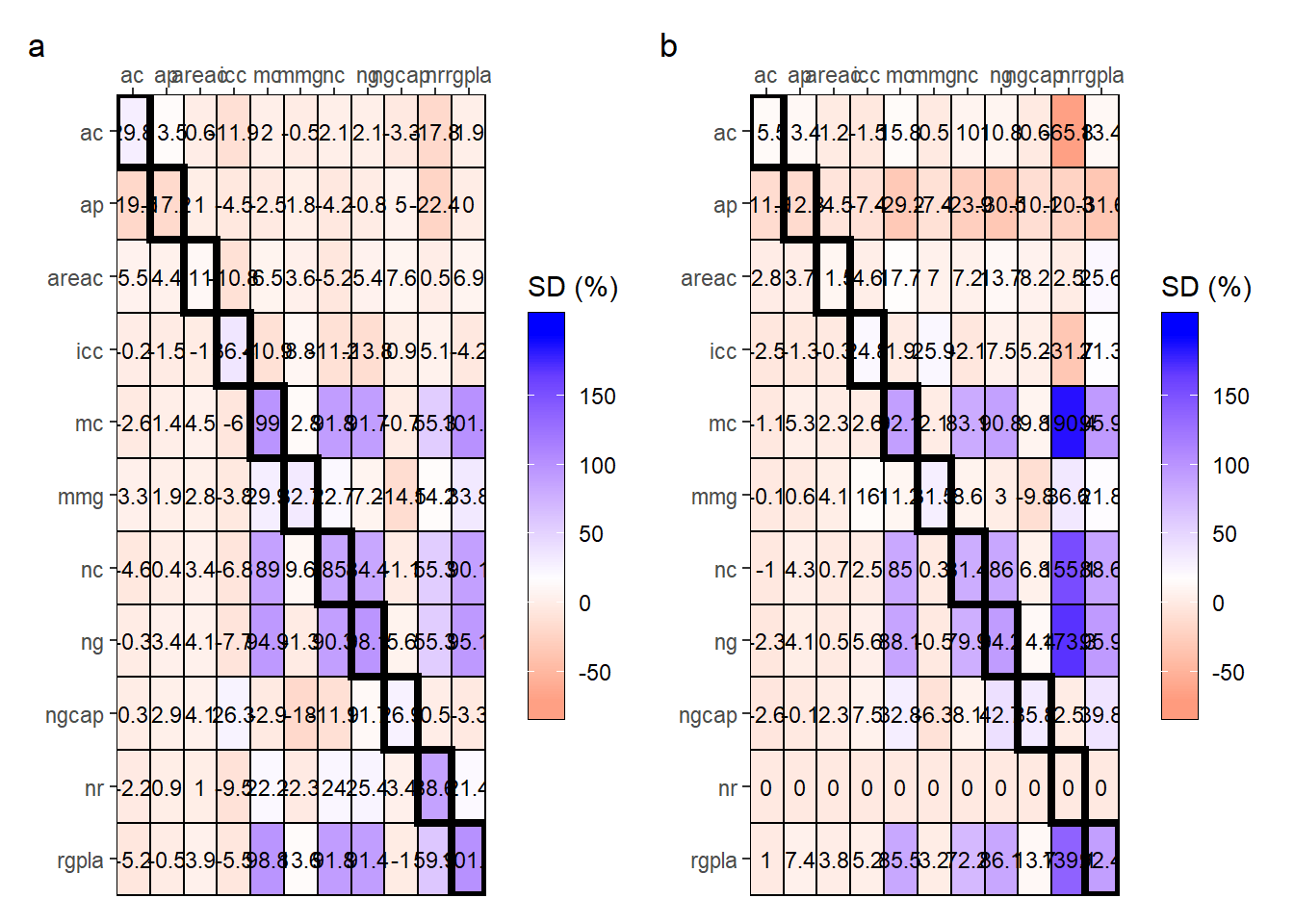
ggsave("figs/direct_indirect_sd.jpg",
       width = 10,
       height = 5)

bind <-
rbind_fill_id(res_epoca$E1$results |> rownames_to_column("var"),
              res_epoca$E2$results |> rownames_to_column("var"),
              .id = "epoca")

# export(bind, "data/sd_absoluto.xlsx")
6 Section info
sessionInfo()
## R version 4.2.2 (2022-10-31 ucrt)
## Platform: x86_64-w64-mingw32/x64 (64-bit)
## Running under: Windows 10 x64 (build 22621)
##
## Matrix products: default
##
## locale:
## [1] LC_COLLATE=Portuguese_Brazil.utf8  LC_CTYPE=Portuguese_Brazil.utf8
## [3] LC_MONETARY=Portuguese_Brazil.utf8 LC_NUMERIC=C
## [5] LC_TIME=Portuguese_Brazil.utf8
##
## attached base packages:
## [1] stats     graphics  grDevices utils     datasets  methods   base
##
## other attached packages:
##  [1] ggridges_0.5.4  metan_1.18.0    lubridate_1.9.2 forcats_1.0.0
##  [5] stringr_1.5.0   dplyr_1.1.2     purrr_1.0.1     readr_2.1.4
##  [9] tidyr_1.3.0     tibble_3.2.1    ggplot2_3.4.2   tidyverse_2.0.0
## [13] rio_0.5.29
##
## loaded via a namespace (and not attached):
##  [1] jsonlite_1.8.7      splines_4.2.2       cellranger_1.1.0
##  [4] yaml_2.3.7          ggrepel_0.9.3       numDeriv_2016.8-1.1
##  [7] pillar_1.9.0        lattice_0.20-45     glue_1.6.2
## [10] digest_0.6.33       RColorBrewer_1.1-3  polyclip_1.10-4
## [13] minqa_1.2.5         colorspace_2.1-0    htmltools_0.5.5
## [16] Matrix_1.6-0        plyr_1.8.8          pkgconfig_2.0.3
## [19] haven_2.5.3         patchwork_1.1.2     scales_1.2.1
## [22] tweenr_2.0.2        openxlsx_4.2.5.2    tzdb_0.4.0
## [25] lme4_1.1-34         ggforce_0.4.1       timechange_0.2.0
## [28] generics_0.1.3      farver_2.1.1        withr_2.5.0
## [31] cli_3.6.1           magrittr_2.0.3      readxl_1.4.3
## [34] evaluate_0.21       GGally_2.1.2        fansi_1.0.4
## [37] nlme_3.1-160        MASS_7.3-60         foreign_0.8-83
## [40] textshaping_0.3.6   tools_4.2.2         data.table_1.14.8
## [43] hms_1.1.3           lifecycle_1.0.3     munsell_0.5.0
## [46] zip_2.3.0           compiler_4.2.2      systemfonts_1.0.4
## [49] rlang_1.1.1         grid_4.2.2          nloptr_2.0.3
## [52] rstudioapi_0.15.0   htmlwidgets_1.6.2   labeling_0.4.2
## [55] rmarkdown_2.23      boot_1.3-28         gtable_0.3.3
## [58] lmerTest_3.1-3      reshape_0.8.9       curl_5.0.1
## [61] R6_2.5.1            knitr_1.43          fastmap_1.1.1
## [64] utf8_1.2.3          mathjaxr_1.6-0      ragg_1.2.5
## [67] stringi_1.7.12      Rcpp_1.0.11         vctrs_0.6.3
## [70] tidyselect_1.2.0    xfun_0.39