03: Seleção multivariada de genótipos de linho usando o índice MGIDI
1 Pacotes
2 Dados
3 Índice MGIDI
mod_mgidi <-
  df |>
  mgidi(ideotype = c("l, h, h, h, h, h, h,  h, h"),
        weights = c(2, 5, 5, 1, 1, 5, 5, 2, 2),
        SI = 25)
##
## -------------------------------------------------------------------------------
## Principal Component Analysis
## -------------------------------------------------------------------------------
## # A tibble: 9 × 4
##   PC    Eigenvalues `Variance (%)` `Cum. variance (%)`
##   <chr>       <dbl>          <dbl>               <dbl>
## 1 PC1          4.43          49.2                 49.2
## 2 PC2          1.72          19.1                 68.3
## 3 PC3          1.03          11.4                 79.8
## 4 PC4          0.94          10.4                 90.2
## 5 PC5          0.62           6.86                97.1
## 6 PC6          0.23           2.56                99.6
## 7 PC7          0.02           0.24                99.9
## 8 PC8          0.01           0.11               100.
## 9 PC9          0              0.02               100
## -------------------------------------------------------------------------------
## Factor Analysis - factorial loadings after rotation-
## -------------------------------------------------------------------------------
## # A tibble: 9 × 6
##   VAR     FA1   FA2   FA3 Communality Uniquenesses
##   <chr> <dbl> <dbl> <dbl>       <dbl>        <dbl>
## 1 cp     0.13 -0.13  0.78        0.65         0.35
## 2 nc    -0.9   0.13 -0.32        0.93         0.07
## 3 ng    -0.93 -0.12 -0.27        0.95         0.05
## 4 areac -0.55 -0.18  0.31        0.44         0.56
## 5 nr    -0.32 -0.18 -0.67        0.58         0.42
## 6 mc    -0.95  0.11 -0.25        0.97         0.03
## 7 rgpla -0.95  0.12 -0.23        0.97         0.03
## 8 ngcap -0.18 -0.92  0.08        0.88         0.12
## 9 mmg   -0.24  0.86  0.06        0.81         0.19
## -------------------------------------------------------------------------------
## Comunalit Mean: 0.7976177
## -------------------------------------------------------------------------------
## Selection differential
## -------------------------------------------------------------------------------
## # A tibble: 9 × 8
##   VAR   Factor      Xo      Xs       SD SDperc sense     goal
##   <chr> <chr>    <dbl>   <dbl>    <dbl>  <dbl> <chr>    <dbl>
## 1 nc    FA1     33.5    59.8    26.2    78.3   increase   100
## 2 ng    FA1    216.    390.    174.     80.3   increase   100
## 3 areac FA1      0.394   0.423   0.0286  7.24  increase   100
## 4 mc    FA1      1.64    3.12    1.48   90.8   increase   100
## 5 rgpla FA1      1.22    2.36    1.15   94.1   increase   100
## 6 ngcap FA2      6.47    6.51    0.0449  0.694 increase   100
## 7 mmg   FA2      5.60    6.50    0.906  16.2   increase   100
## 8 cp    FA3     27.6    26.5    -1.09   -3.95  decrease   100
## 9 nr    FA3      1.29    1.69    0.400  31.0   increase   100
## ------------------------------------------------------------------------------
## Selected genotypes
## -------------------------------------------------------------------------------
## G228 G4 G48 G13 G222 G31 G9 G36 G28 G29 G10 G21 G23 G41 G14 G17
## -------------------------------------------------------------------------------
plot(mod_mgidi)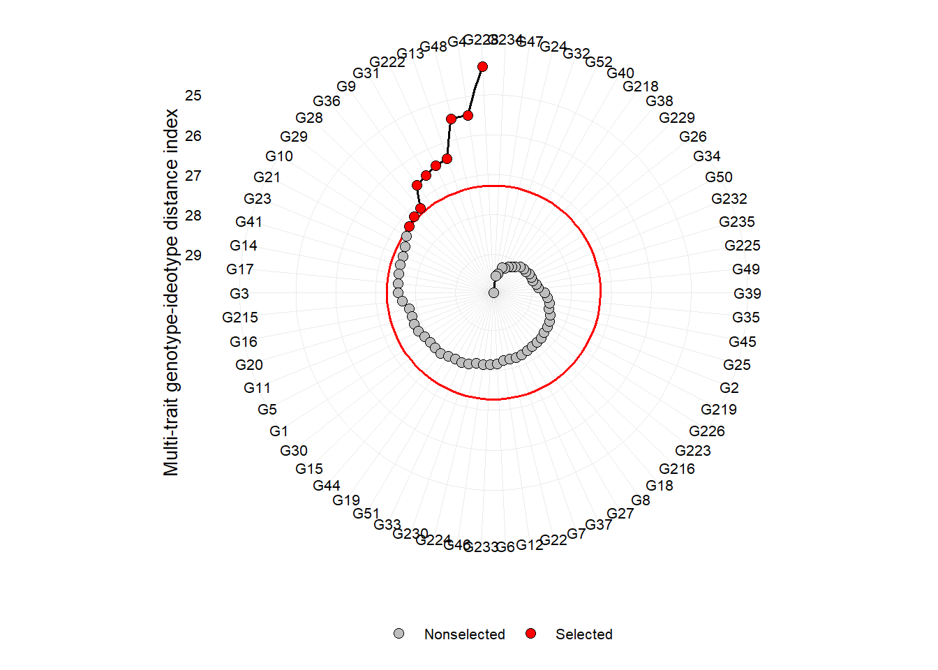
# ggsave("figs/mgidi")
plot(mod_mgidi, type  = "contribution")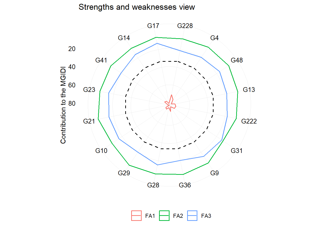
df_plot <-
  gmd(mod_mgidi) %>%
  select_cols(VAR, Xo, Xs, SDperc, sense) %>%
  mutate(strategy = "Multivariado") |>
  replace_string(sense, pattern = "increase", replacement = "Positivo desejado") |>
  replace_string(sense, pattern = "decrease", replacement = "Negativo desejado")
4 Seleção univariada para RG
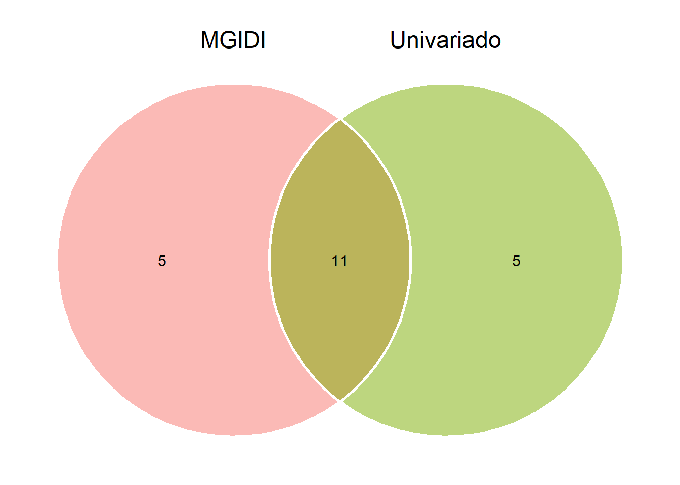
sel_uni <- muni <- df |> slice_max(rgpla, n = 16)

muni <-
  sel_uni |>
  mean_by() |>
  pivot_longer(cols = everything(),
               values_to = "Xs",
               names_to = "VAR")

mger <-
  df |>
  mean_by() |>
  pivot_longer(cols = everything(),
               values_to = "Xo",
               names_to = "VAR")

sd_uni <-
  left_join(mger, muni) |>
  mutate(SDperc = (Xs - Xo) / Xo * 100) |>
  left_join(df_plot |> select(VAR, sense)) |>
  mutate(strategy = "Univariado")

df_plot2 <-
  bind_rows(df_plot, sd_uni)
ggplot(df_plot2, aes(SDperc, VAR)) +
  geom_col(position = position_dodge(),
           aes(fill = sense),
           width = 1,
           linewidth = 0.1,
           color = "black") +
  geom_text(aes(label = round(SDperc, 2),
                hjust = ifelse(SDperc > 0, -0.1, 1.1)),
            size = 4) +
  facet_wrap(~strategy) +
  theme_bw(base_size = 18) +
  theme(axis.text = element_text(size = 12, color = "black"),
        axis.ticks.length = unit(0.2, "cm"),
        panel.grid.minor = element_blank(),
        legend.title = element_blank(),
        legend.position = "bottom",
        panel.spacing.x = unit(0, "cm")) +
  geom_vline(xintercept = 0, linetype = 1, linewidth = 1) +
  scale_x_continuous(expand = expansion(c(0.2, 0.3))) +
  labs(y = "Caracteres avaliados",
       x = "Diferencial de seleção (%)") +
  geom_vline(xintercept = 0)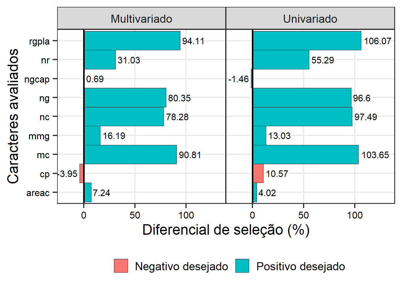
ggsave("figs/gain_mgidi.jpg",
       width = 8,
       height = 5)


plot(mod_mgidi, SI = 25) +
  theme(legend.position = "right")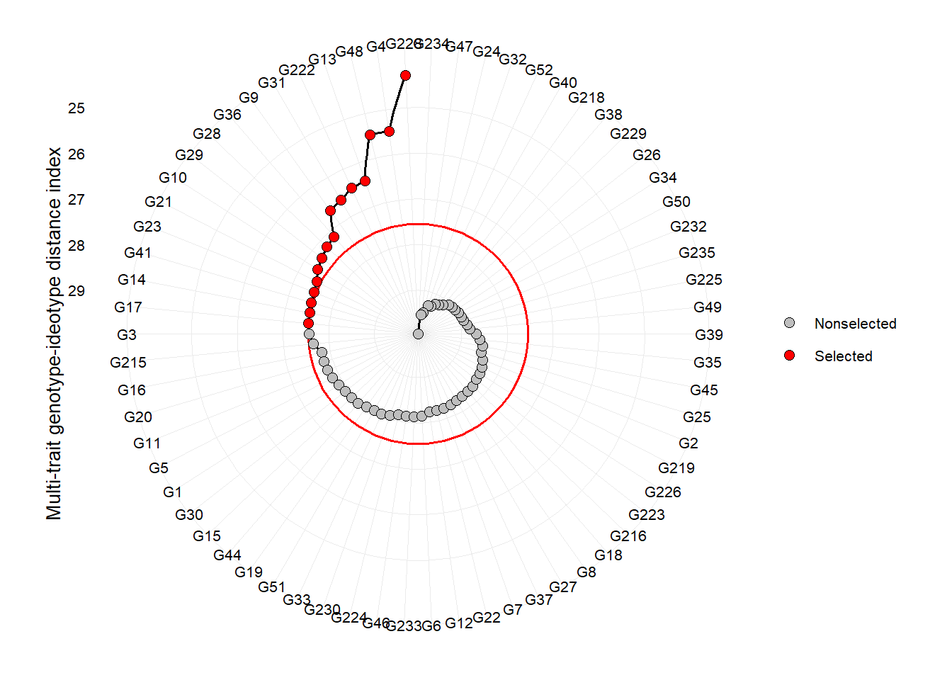
ggsave("figs/mgidi_radar.jpg",
       width = 8,
       height = 7)
5 Histogram
library(ggridges)
df_sel <-
  df |>
  mutate(selecionado = ifelse(gen %in% mod_mgidi$sel_gen, "Selecionado", "Não selecionado"))

library(ggExtra)
library(ggrepel)

p1 <-
ggplot(df_sel, aes(rgpla, mmg, color = selecionado, group = selecionado)) +
  geom_point(size = 2, alpha = 0.7) +
  theme_bw(base_size = 18) +
  geom_text_repel(data = df_sel |>  filter(selecionado == "Selecionado"),
                  aes(label = gen),
                  show.legend = FALSE,
                  size = 3) +
  theme(legend.position = "bottom",
        panel.grid.minor = element_blank())+
  labs(color = "",
       y = "Massa de mil grãos (g)",
       x = "Rendimento de grãos por planta (g)")

ggMarginal(p1, type="boxplot", groupFill = TRUE)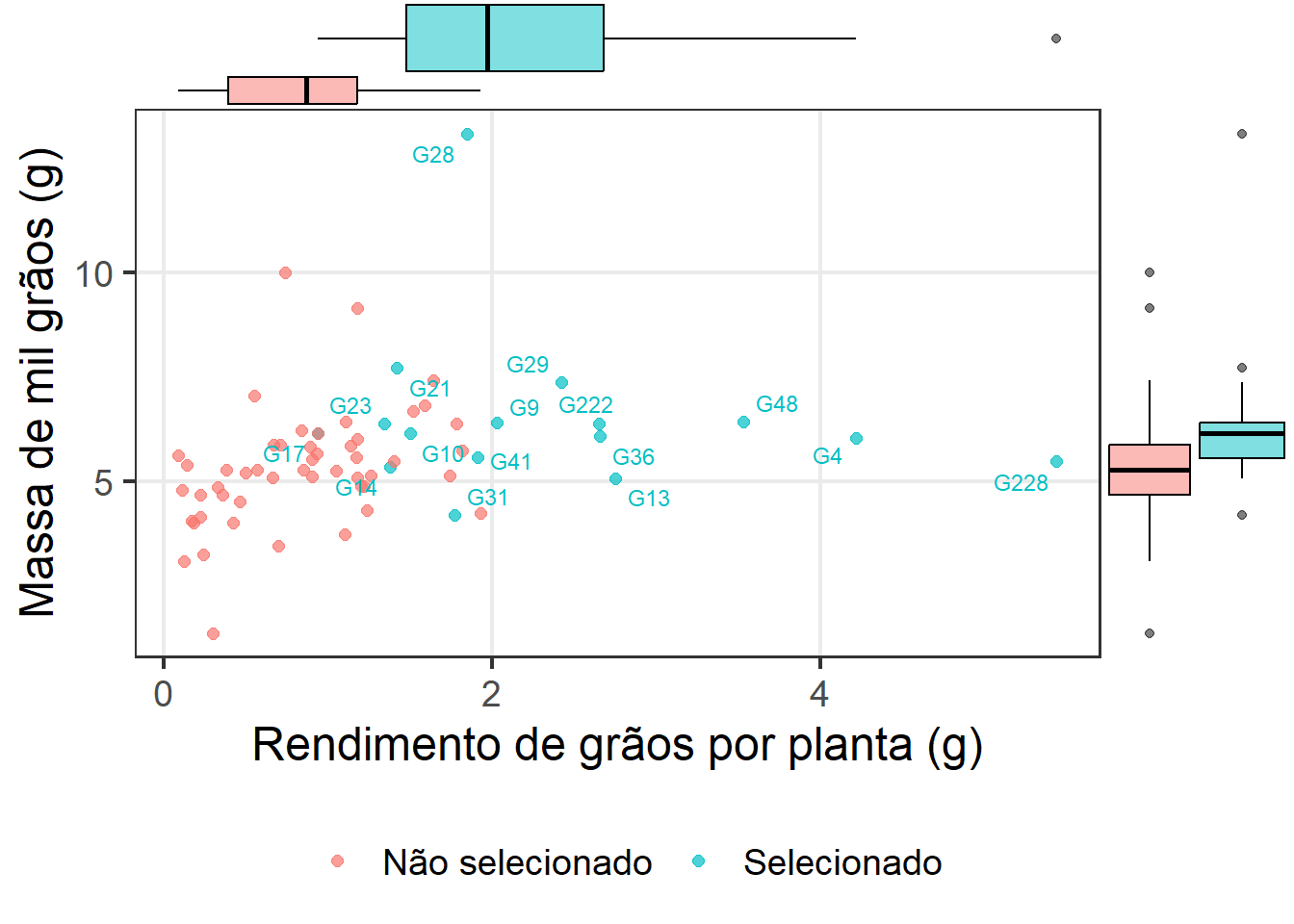
6 Venn plot
7 Section info
sessionInfo()
## R version 4.2.2 (2022-10-31 ucrt)
## Platform: x86_64-w64-mingw32/x64 (64-bit)
## Running under: Windows 10 x64 (build 22621)
##
## Matrix products: default
##
## locale:
## [1] LC_COLLATE=Portuguese_Brazil.utf8  LC_CTYPE=Portuguese_Brazil.utf8
## [3] LC_MONETARY=Portuguese_Brazil.utf8 LC_NUMERIC=C
## [5] LC_TIME=Portuguese_Brazil.utf8
##
## attached base packages:
## [1] stats     graphics  grDevices utils     datasets  methods   base
##
## other attached packages:
##  [1] ggrepel_0.9.3   ggExtra_0.10.0  ggridges_0.5.4  metan_1.18.0
##  [5] lubridate_1.9.2 forcats_1.0.0   stringr_1.5.0   dplyr_1.1.2
##  [9] purrr_1.0.1     readr_2.1.4     tidyr_1.3.0     tibble_3.2.1
## [13] ggplot2_3.4.2   tidyverse_2.0.0 rio_0.5.29
##
## loaded via a namespace (and not attached):
##  [1] nlme_3.1-160        RColorBrewer_1.1-3  numDeriv_2016.8-1.1
##  [4] tools_4.2.2         utf8_1.2.3          R6_2.5.1
##  [7] colorspace_2.1-0    withr_2.5.0         tidyselect_1.2.0
## [10] GGally_2.1.2        curl_5.0.1          compiler_4.2.2
## [13] textshaping_0.3.6   cli_3.6.1           labeling_0.4.2
## [16] scales_1.2.1        systemfonts_1.0.4   digest_0.6.33
## [19] foreign_0.8-83      minqa_1.2.5         rmarkdown_2.23
## [22] pkgconfig_2.0.3     htmltools_0.5.5     lme4_1.1-34
## [25] fastmap_1.1.1       htmlwidgets_1.6.2   rlang_1.1.1
## [28] readxl_1.4.3        rstudioapi_0.15.0   shiny_1.7.4.1
## [31] farver_2.1.1        generics_0.1.3      jsonlite_1.8.7
## [34] zip_2.3.0           magrittr_2.0.3      patchwork_1.1.2
## [37] Matrix_1.6-0        Rcpp_1.0.11         munsell_0.5.0
## [40] fansi_1.0.4         lifecycle_1.0.3     stringi_1.7.12
## [43] yaml_2.3.7          mathjaxr_1.6-0      MASS_7.3-60
## [46] plyr_1.8.8          grid_4.2.2          promises_1.2.0.1
## [49] miniUI_0.1.1.1      lattice_0.20-45     haven_2.5.3
## [52] splines_4.2.2       hms_1.1.3           knitr_1.43
## [55] pillar_1.9.0        boot_1.3-28         glue_1.6.2
## [58] evaluate_0.21       data.table_1.14.8   vctrs_0.6.3
## [61] nloptr_2.0.3        tzdb_0.4.0          tweenr_2.0.2
## [64] httpuv_1.6.11       cellranger_1.1.0    gtable_0.3.3
## [67] polyclip_1.10-4     reshape_0.8.9       xfun_0.39
## [70] ggforce_0.4.1       openxlsx_4.2.5.2    mime_0.12
## [73] xtable_1.8-4        later_1.3.1         ragg_1.2.5
## [76] lmerTest_3.1-3      timechange_0.2.0    ellipsis_0.3.2