04: Modelagem da área foliar de cultivares de linho em diferentes épocas de semeadura utilizando o modelo Logístico
1 Libraries
To reproduce the examples of this material, the R packages the following packages are needed.
2 Data
2.1 Temperature
dft <-
  import("data/clima.csv", dec = ",") |>
  separate(hora, into = c("dia", "mes", "ano")) |>
  unite("data", dia, mes, ano, sep = "/") |>
  mutate(data = dmy(data))

dftemp <-
  dft |>
  group_by(data) |>
  summarise(tmin = min(tmin),
            tmed = mean(tmed),
            tmax = max(tmax),
            prec = sum(prec),
            ur = mean(ur)) |>
  mutate(gd = tmed - 5,
         gd2 = ((tmax + tmin) / 2) - 5) |>
  mutate(data = ymd(data))

dftempe1 <-
  dftemp |>
  slice(1:79) |>
  mutate(epoca = "E1")

dftempe2 <-
  dftemp |>
  slice(79:148) |>
  mutate(epoca = "E2")

dftemp2 <-
  bind_rows(dftempe1, dftempe2) |>
  relocate(epoca, .before = data) |>
  group_by(epoca) |>
  mutate(gda = cumsum(gd),
         gda2 = cumsum(gd2)) |>
  separate(data, into = c("ano", "mes", "dia")) |>
  unite("data", dia, mes, sep = "/")

# GRAUS DIA
df
## function (x, df1, df2, ncp, log = FALSE)
## {
##     if (missing(ncp))
##         .Call(C_df, x, df1, df2, log)
##     else .Call(C_dnf, x, df1, df2, ncp, log)
## }
## <bytecode: 0x00000285622e1f10>
## <environment: namespace:stats>
2.2 gráfico densidade
library(ggridges)
dft |>
  separate(data, into = c("ano", "mes", "dia")) |>
  ggplot(aes(x = tmax, y = mes, fill = after_stat(x))) +
  geom_density_ridges_gradient() +
  scale_fill_viridis_c() +
  labs(x = "Temperatura média (ºC)",
       y = "Meses do ano",
       fill = "Temperatura\nmédia (ºC)")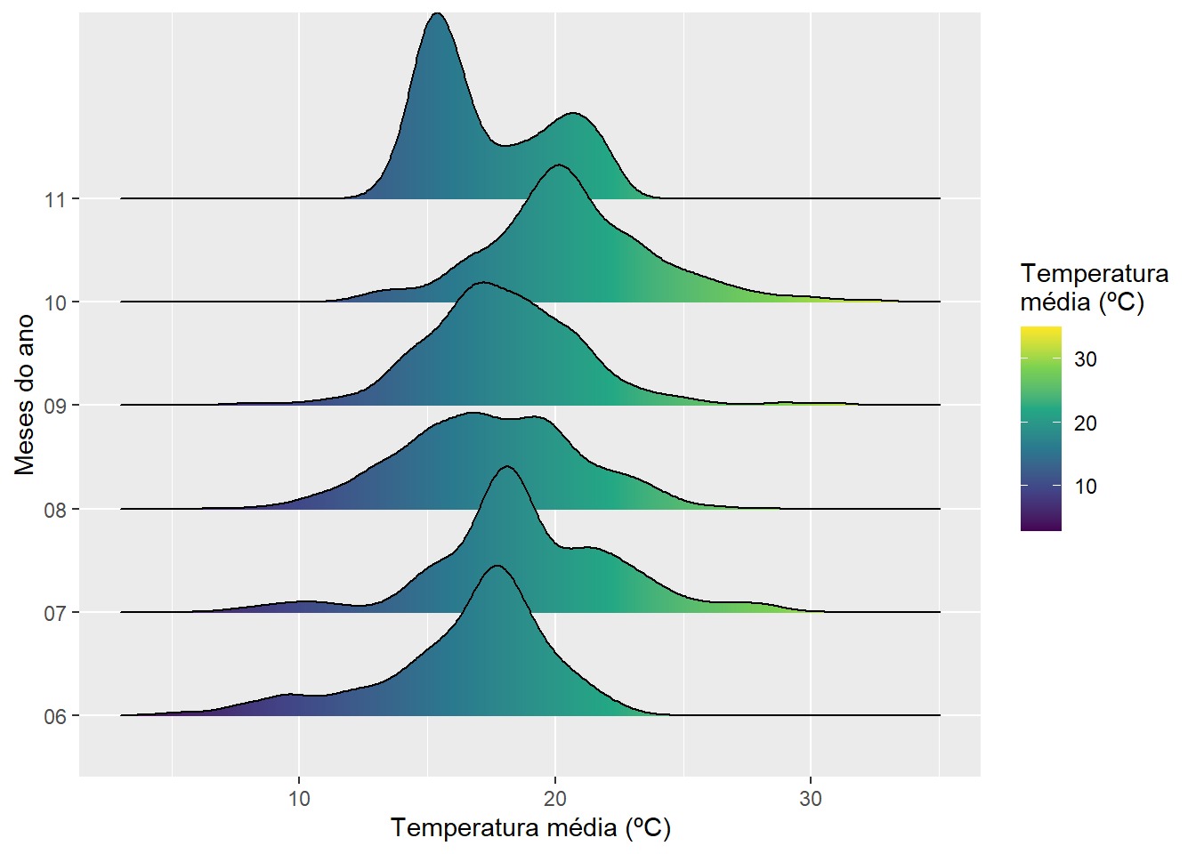
2.3 Gráfico
ggplot() +
  geom_bar(dftemp,
           mapping = aes(x = data, y = prec * 30 / 100),
           stat = "identity",
           fill = "skyblue") +
  geom_line(dftemp,
            mapping = aes(x = data, y = tmax, colour = "red"),
            linewidth = 1,
            alpha = 0.1) +
  geom_line(dftemp,
            mapping = aes(x = data, y = tmin, colour = "blue"),
            linewidth = 1,
            alpha = 0.1) +
  geom_smooth(dftemp,
              mapping = aes(x = data, y = tmax, colour = "red"),
              linewidth = 1,
              se = FALSE) +
  geom_smooth(dftemp,
              mapping = aes(x = data, y = tmin, colour = "blue"),
              linewidth = 1,
              se = FALSE) +
  scale_x_date(date_breaks = "15 days", date_labels =  "%d/%m",
               expand = expansion(c(0, 0)))+
  scale_y_continuous(name = expression("Temperatura ("~degree~"C)"),
                     sec.axis = sec_axis(~ . * 100 / 30 , name = "Precipitação (mm)")) +
  theme(legend.position = "bottom",
        legend.title = element_blank(),
        axis.text.x = element_text(angle = 45, vjust = 1, hjust = 1)) +
  scale_color_identity(breaks = c("red", "blue"),
                       labels = c("Temperatura máxima (ºC)",
                                  "Temperatura mínima (ºC)"),
                       guide = "legend") +
  labs(x = "Dia do ano",
       color = "") +
  theme_bw(base_size = 16) +
  theme(
    panel.grid.major = element_blank(), #remove major gridlines
    # panel.grid.minor = element_blank(), #remove minor gridlines
    legend.background = element_rect(fill='transparent'), #transparent legend bg
    legend.position = "bottom") #transparent legend panel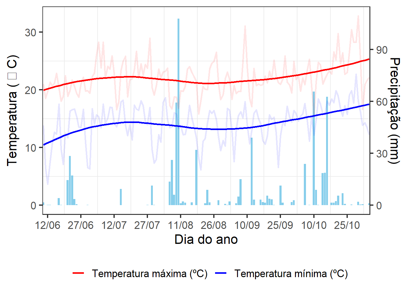
ggsave("figs/temperature.jpg",
       width = 12,
       height = 8)
3 modelo
df_model <- import("data/df_model_cresc.xlsx")

formula <- af_planta ~ b1/(1 + exp(b2 - b3 * gda))
start_af = c(b1 = 60,
             b2 = 6,
             b3 = 0.02)
mod_af <-
  df_model |>
  filter(data != "04/11") |>
  group_by(epoca, cultivar, bloco) |>
  doo(~nls(formula,
           data = .,
           start = start_af))

parameters <-
  mod_af |>
  mutate(data = map(data, ~.x |> tidy())) |>
  unnest(data) |>
  select(epoca, cultivar, bloco, term, estimate) |>
  pivot_wider(names_from = term,
              values_from = estimate)
4 ANOVA
# ANOVAS
mod_anova <-
  mod_af |>
  mutate(data = map(data, ~.x |> tidy())) |>
  unnest(data) |>
  select(epoca, cultivar, bloco, term, estimate) |>
  rename(parameter = term) |>
  group_by(parameter) %>%
  doo(~aov(estimate ~ epoca*cultivar + bloco, data = .))


# TABELA ANOVA
tab_anova <-
  mod_anova |>
  mutate(data = map(data, ~.x |> tidy())) |>
  unnest(data)
tab_anova
## # A tibble: 15 × 7
##    parameter term              df   sumsq  meansq statistic  p.value
##    <chr>     <chr>          <dbl>   <dbl>   <dbl>     <dbl>    <dbl>
##  1 b1        epoca              1 2.93e+3 2.93e+3  16.3      0.00686
##  2 b1        cultivar           1 1.66e+3 1.66e+3   9.21     0.0229
##  3 b1        bloco              2 5.79e+2 2.89e+2   1.61     0.276
##  4 b1        epoca:cultivar     1 2.42e+2 2.42e+2   1.34     0.291
##  5 b1        Residuals          6 1.08e+3 1.80e+2  NA       NA
##  6 b2        epoca              1 6.67e+0 6.67e+0  33.2      0.00119
##  7 b2        cultivar           1 2.01e-1 2.01e-1   1.00     0.356
##  8 b2        bloco              2 8.91e-1 4.46e-1   2.22     0.190
##  9 b2        epoca:cultivar     1 3.95e-1 3.95e-1   1.96     0.211
## 10 b2        Residuals          6 1.21e+0 2.01e-1  NA       NA
## 11 b3        epoca              1 3.29e-7 3.29e-7   0.0995   0.763
## 12 b3        cultivar           1 1.34e-7 1.34e-7   0.0406   0.847
## 13 b3        bloco              2 2.57e-5 1.29e-5   3.88     0.0828
## 14 b3        epoca:cultivar     1 1.22e-8 1.22e-8   0.00367  0.954
## 15 b3        Residuals          6 1.99e-5 3.31e-6  NA       NA

# export(tab_anova, "data/result_logistico.xlsx", which = "anova_par")


# comparação de médias
mcomp_cult <-
  mod_anova |>
  mutate(data = map(data, ~.x |> emmeans(~cultivar)))
mcomp_epoca <-
  mod_anova |>
  mutate(data = map(data, ~.x |> emmeans(~epoca)))


# beta1
b1e <-
  plot(mcomp_epoca$data[[1]], comparisons = TRUE, CIs = FALSE) +
  labs(x = expression(beta[1]),
       y = "Época") +
  theme_bw(base_size = 14) +
  xlim(c(60, 100))
b1c <-
  plot(mcomp_cult$data[[1]], comparisons = TRUE, CIs = FALSE) +
    labs(x = expression(beta[1]),
       y = "Cultivar") +
  theme_bw(base_size = 14)+
  xlim(c(60, 100))

# beta2 (epoca)
b2e <-
  plot(mcomp_epoca$data[[2]], comparisons = TRUE, CIs = FALSE) +
    labs(x = expression(beta[2]),
       y = "Época") +
  theme_bw(base_size = 14)

arrange_ggplot(b1e, b1c, b2e,
               ncol = 1,
               tag_levels = "a")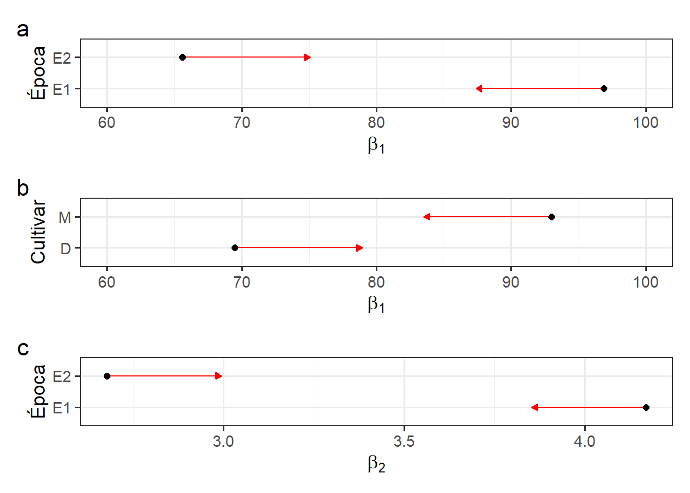
ggsave("figs/anova_pars.jpg",
       height = 5,
       width = 4)
4.1 Qualidade de ajuste
library(hydroGOF)
get_r2 <- function(model){
  aic <- AIC(model)
  fit <- model$m$fitted()
  res <- model$m$resid()
  obs <- fit + res
  gof <- gof(obs, fit, digits = 4)
  r2 <- gof[which(rownames(gof) == "R2")]
  data.frame(aic = aic, r2 = r2)
}

qualidade <-
  mod_af |>
  mutate(map_dfr(.x = data,
                 .f = ~get_r2(.))) |>
  select(-data)

# export(qualidade, "data/result_logistico.xlsx", which = "qualidade")
5 Modelo ajustado
# área foliar
formula <- y ~ b1/(1 + exp(b2 - b3 * x))

# a <-
ggplot(df_model |> filter(!data %in% c("04/11")),
       aes(gda, af_planta, color = cultivar)) +
  geom_smooth(method = "nls",
              method.args = list(formula = formula,
                                 start = c(b1 = 60,
                                           b2 = 2,
                                           b3 = 0.02)),
              se = FALSE,
              aes(color = cultivar)) +
  facet_wrap(~epoca) +
  stat_summary(fun = mean,
               geom = "point",
               aes(color = cultivar),
               size = 2.5,
               position = position_dodge(width = 0.8)) +
  scale_y_continuous(breaks = seq(0, 150, by = 25)) +
  labs(x = "Graus dia acumulado",
       y = expression(Área~foliar~média~(cm^2~planta^{-1}))) +
  scale_color_manual(values = c("gold", "brown")) +
  stat_summary(data = df_model |>  filter(data == "04/11"),
               aes(x = gda, y = af_planta),
               fun = mean,
               alpha = 0.4,
               shape = 16,
               show.legend = FALSE) +
  theme_bw(base_size = 20) +
  theme(
    panel.grid.major = element_blank(), #remove major gridlines
    # panel.grid.minor = element_blank(), #remove minor gridlines
    legend.background = element_rect(fill='transparent'), #transparent legend bg
    legend.position = "bottom") #transparent legend panel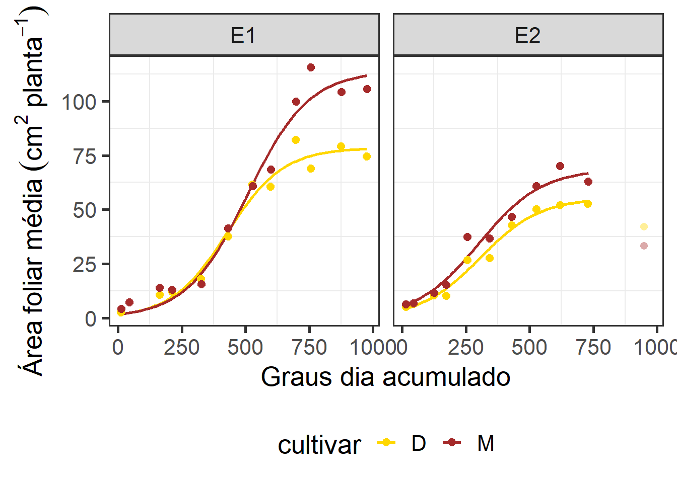
ggsave("figs/mod_logistico.jpg",
       width = 9,
       height = 5)
5.1 Primeira derivada
# primeira derivada
D(expression(b1/(1 + exp(b2 - b3 * das))), "das")
## b1 * (exp(b2 - b3 * das) * b3)/(1 + exp(b2 - b3 * das))^2

dy <- function(x,b1,b2,b3){
  b1 * (exp(b2 - b3 * x) * b3)/(1 + exp(b2 - b3 * x))^2
}

parameters <-
  parameters |>
  mean_by(epoca, cultivar) |>
  mutate(xpi = b2 / b3,
         ypi = dy(xpi, b1, b2, b3)) |>
  as.data.frame()

# plot_pi <-
ggplot() +
  stat_function(fun = dy,
                aes(color = "D", linetype = "E1"),
                n = 500,
                linewidth = 1,
                xlim = c(0, 1000),
                args = c(b1 = parameters[[1, 3]],
                         b2 = parameters[[1, 4]],
                         b3 = parameters[[1, 5]])) +
  stat_function(fun = dy,
                aes(color = "M", linetype = "E1"),
                linewidth = 1,
                xlim = c(0, 1000),
                args = c(b1 = parameters[[2, 3]],
                         b2 = parameters[[2, 4]],
                         b3 = parameters[[2, 5]])) +
  stat_function(fun = dy,
                aes(color = "D", linetype = "E2"),
                linewidth = 1,
                xlim = c(0, 1000),
                args = c(b1 = parameters[[3, 3]],
                         b2 = parameters[[3, 4]],
                         b3 = parameters[[3, 5]])) +
  stat_function(fun = dy,
                aes(color = "M", linetype = "E2"),
                linewidth = 1,
                xlim = c(0, 1000),
                args = c(b1 = parameters[[4, 3]],
                         b2 = parameters[[4, 4]],
                         b3 = parameters[[4, 5]])) +
  geom_point(aes(xpi, ypi, shape = epoca, color = cultivar),
             data = parameters,
             size = 3,
             show.legend = FALSE) +
  theme_bw(base_size = 22) +
  scale_x_continuous(breaks = seq(0, 1200, by = 200)) +
  labs(x = "Graus dia acumulado",
       y = expression(Emissão~de~área~foliar~(cm^2~planta^{-1}~grau~dia^{-1})),
       color  = "Cultivar",
       linetype = "Época") +
  theme(legend.position = "bottom",
        panel.grid.minor = element_blank()) +
  scale_color_manual(values = c("gold", "brown"))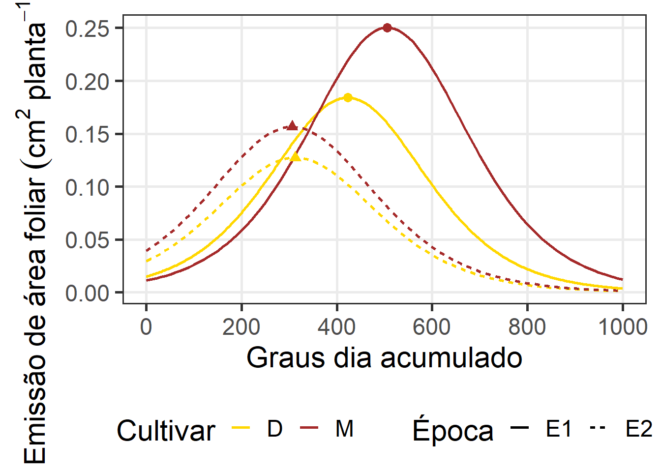
ggsave("figs/prim_deriv.jpg",
       height = 8,
       width = 8)
5.2 Segunda derivada
# segunda derivada
D(expression(b1 * (exp(b2 - b3 * x) * b3)/(1 + exp(b2 - b3 * x))^2), "x")
## -(b1 * (exp(b2 - b3 * x) * b3 * b3)/(1 + exp(b2 - b3 * x))^2 -
##     b1 * (exp(b2 - b3 * x) * b3) * (2 * (exp(b2 - b3 * x) * b3 *
##         (1 + exp(b2 - b3 * x))))/((1 + exp(b2 - b3 * x))^2)^2)

d2y <- function(x,b1,b2,b3){
  -(b1 * (exp(b2 - b3 * x) * b3 * b3)/(1 + exp(b2 - b3 * x))^2 -
      b1 * (exp(b2 - b3 * x) * b3) * (2 * (exp(b2 - b3 * x) * b3 *
                                             (1 + exp(b2 - b3 * x))))/((1 + exp(b2 - b3 * x))^2)^2)
}

parameters <-
  parameters |>
  mutate(xmap = (b2 - 1.3170)/b3,
         xmdp = (b2 + 1.3170)/b3,
         ymap = d2y(xmap, b1, b2, b3),
         ymdp = d2y(xmdp, b1, b2, b3),
  )


# df_acel <-
ggplot() +
  geom_hline(yintercept = 0) +
  stat_function(fun = d2y,
                aes(color = "D", linetype = "E1"),
                n = 500,
                linewidth = 1,
                xlim = c(0, 1000),
                args = c(b1 = parameters[[1, 3]],
                         b2 = parameters[[1, 4]],
                         b3 = parameters[[1, 5]])) +
  stat_function(fun = d2y,
                aes(color = "M", linetype = "E1"),
                linewidth = 1,
                xlim = c(0, 1000),
                args = c(b1 = parameters[[2, 3]],
                         b2 = parameters[[2, 4]],
                         b3 = parameters[[2, 5]])) +
  stat_function(fun = d2y,
                aes(color = "D", linetype = "E2"),
                linewidth = 1,
                xlim = c(0, 1000),
                args = c(b1 = parameters[[3, 3]],
                         b2 = parameters[[3, 4]],
                         b3 = parameters[[3, 5]])) +
  stat_function(fun = d2y,
                aes(color = "M", linetype = "E2"),
                linewidth = 1,
                xlim = c(0, 1000),
                args = c(b1 = parameters[[4, 3]],
                         b2 = parameters[[4, 4]],
                         b3 = parameters[[4, 5]])) +
  geom_point(aes(xmap, ymap, fill = cultivar),
             data = parameters,
             size = 3,
             shape = 24,
             show.legend = FALSE) +
  geom_point(aes(xmdp, ymdp, fill = cultivar),
             data = parameters,
             size = 3,
             shape = 25,
             show.legend = FALSE) +
  theme_bw(base_size = 22) +
  labs(x = "Graus dia acumulado",
       y = expression(Aceleração~(cm^2~planta^{-1}~grau~dia^{-2})),
       color  = "Cultivar",
       linetype = "Época") +
    theme(legend.position = "bottom",
        panel.grid.minor = element_blank()) +
  scale_color_manual(values = c("gold", "brown")) +
  scale_fill_manual(values = c("gold", "brown"))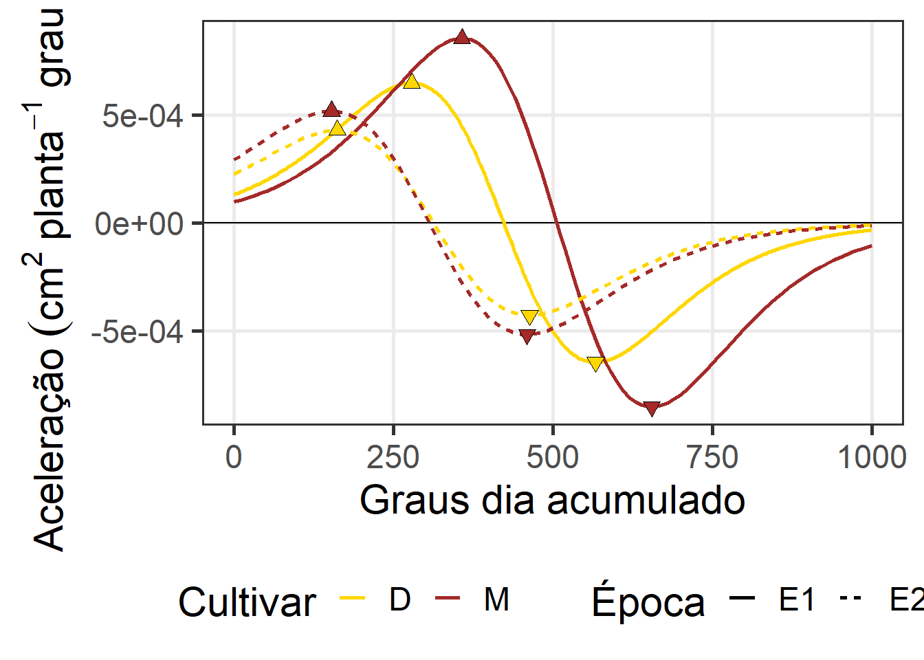
ggsave("figs/seg_deriv.jpg",
       height = 8,
       width = 8)

# export(parameters, "data/result_logistico.xlsx", which = "parametros_logistico")
6 Section info
sessionInfo()
## R version 4.2.2 (2022-10-31 ucrt)
## Platform: x86_64-w64-mingw32/x64 (64-bit)
## Running under: Windows 10 x64 (build 22621)
##
## Matrix products: default
##
## locale:
## [1] LC_COLLATE=Portuguese_Brazil.utf8  LC_CTYPE=Portuguese_Brazil.utf8
## [3] LC_MONETARY=Portuguese_Brazil.utf8 LC_NUMERIC=C
## [5] LC_TIME=Portuguese_Brazil.utf8
##
## attached base packages:
## [1] stats     graphics  grDevices utils     datasets  methods   base
##
## other attached packages:
##  [1] hydroGOF_0.4-0  zoo_1.8-12      ggridges_0.5.4  emmeans_1.8.7
##  [5] broom_1.0.5     metan_1.18.0    lubridate_1.9.2 forcats_1.0.0
##  [9] stringr_1.5.0   dplyr_1.1.2     purrr_1.0.1     readr_2.1.4
## [13] tidyr_1.3.0     tibble_3.2.1    ggplot2_3.4.2   tidyverse_2.0.0
## [17] rio_0.5.29
##
## loaded via a namespace (and not attached):
##   [1] TH.data_1.1-2       minqa_1.2.5         colorspace_2.1-0
##   [4] class_7.3-20        estimability_1.4.1  rstudioapi_0.15.0
##   [7] proxy_0.4-27        farver_2.1.1        ggrepel_0.9.3
##  [10] fansi_1.0.4         mvtnorm_1.2-2       mathjaxr_1.6-0
##  [13] codetools_0.2-18    splines_4.2.2       knitr_1.43
##  [16] polyclip_1.10-4     jsonlite_1.8.7      nloptr_2.0.3
##  [19] ggforce_0.4.1       compiler_4.2.2      backports_1.4.1
##  [22] Matrix_1.6-0        fastmap_1.1.1       cli_3.6.1
##  [25] tweenr_2.0.2        htmltools_0.5.5     tools_4.2.2
##  [28] lmerTest_3.1-3      coda_0.19-4         gtable_0.3.3
##  [31] glue_1.6.2          Rcpp_1.0.11         cellranger_1.1.0
##  [34] vctrs_0.6.3         nlme_3.1-160        lwgeom_0.2-13
##  [37] xfun_0.39           openxlsx_4.2.5.2    lme4_1.1-34
##  [40] timechange_0.2.0    lifecycle_1.0.3     MASS_7.3-60
##  [43] scales_1.2.1        gstat_2.1-1         ragg_1.2.5
##  [46] hms_1.1.3           parallel_4.2.2      sandwich_3.0-2
##  [49] RColorBrewer_1.1-3  yaml_2.3.7          curl_5.0.1
##  [52] reshape_0.8.9       stringi_1.7.12      maptools_1.1-7
##  [55] e1071_1.7-13        boot_1.3-28         zip_2.3.0
##  [58] intervals_0.15.4    rlang_1.1.1         pkgconfig_2.0.3
##  [61] systemfonts_1.0.4   evaluate_0.21       lattice_0.20-45
##  [64] sf_1.0-13           patchwork_1.1.2     htmlwidgets_1.6.2
##  [67] labeling_0.4.2      tidyselect_1.2.0    GGally_2.1.2
##  [70] hydroTSM_0.6-0      plyr_1.8.8          magrittr_2.0.3
##  [73] R6_2.5.1            generics_0.1.3      automap_1.1-9
##  [76] multcomp_1.4-25     DBI_1.1.3           pillar_1.9.0
##  [79] haven_2.5.3         foreign_0.8-83      withr_2.5.0
##  [82] mgcv_1.8-41         stars_0.6-1         units_0.8-2
##  [85] xts_0.13.1          abind_1.4-5         survival_3.4-0
##  [88] sp_2.0-0            spacetime_1.3-0     KernSmooth_2.23-20
##  [91] utf8_1.2.3          tzdb_0.4.0          rmarkdown_2.23
##  [94] grid_4.2.2          readxl_1.4.3        data.table_1.14.8
##  [97] FNN_1.1.3.2         classInt_0.4-9      digest_0.6.33
## [100] xtable_1.8-4        numDeriv_2016.8-1.1 textshaping_0.3.6
## [103] munsell_0.5.0       viridisLite_0.4.2