10. Um método simples e indireto para estimação da área de folha de linho

% Analysis

1 Libraries

To reproduce the examples of this material, the R packages the following packages are needed.

library(pliman)
library(caret)
library(doParallel)
library(tidyverse)
library(DescTools)
library(ggExtra)
library(performance)

2 Data

df_af <- rio::import("data/leaf_flax_pred.xlsx")
descritiva <- 
  df_af |> 
  summarise(across(area:width, .fns = list(media = mean, min = min, max = max)))

descritiva
##   area_media   area_min area_max length_media length_min length_max width_media
## 1  0.5909433 0.04281334 1.907076     2.142723   0.511989    4.37025   0.3322159
##    width_min width_max
## 1 0.09535828 0.5995659

p1 <- 
ggplot(df_af, aes(length, area)) + 
  geom_point( size = 3, alpha = 0.5, color = "brown") +
  labs(x = "Comprimento da folha (cm)",
       y = expression(Área~foliar~(cm^2~folha^{-1}))) +
  theme_bw(base_size = 16)
ggMarginal(p1, color = "brown", size = 7, linewidth = 1)


p2 <- 
ggplot(df_af, aes(width, area)) + 
  geom_point( size = 3, alpha = 0.5, color = "brown") +
  labs(x = "Largura da folha (cm)",
       y = expression(Área~foliar~(cm^2~folha^{-1}))) +
  theme_bw(base_size = 16)
ggMarginal(p2, color = "brown", size = 7, linewidth = 1)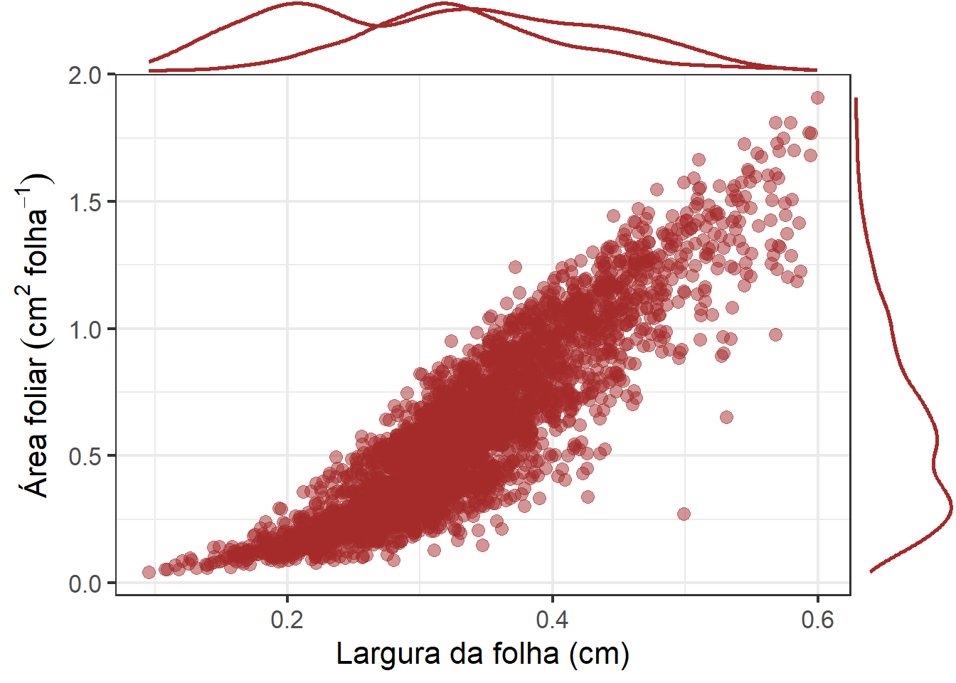

# functions
# concordance correlation coefficient
get_ccc <- function(df, predicted, real){
  if(is.grouped_df(df)){
    df %>% 
      group_modify(~get_ccc(.x, {{predicted}}, {{real}})) %>% 
      ungroup()
  } else{
    predicted <- pull(df, {{predicted}})
    real <- pull(df, {{real}})
    cor <- CCC(real, predicted, na.rm = TRUE)
    data.frame(r = cor(real, predicted),
               pc = cor$rho.c[[1]],
               lwr_ci = cor$rho.c[[2]],
               upr_ci = cor$rho.c[[3]],
               bc = cor$C.b)
  }
}

3 Model

control <-
  trainControl(method = 'cv',
               p = 0.7,
               number = 10,
               verboseIter = TRUE,
               savePredictions = "all")

fit <- train(area ~  length + length:width ,
             method = "lm",
             data = df_af,
             trControl = control)
## + Fold01: intercept=TRUE 
## - Fold01: intercept=TRUE 
## + Fold02: intercept=TRUE 
## - Fold02: intercept=TRUE 
## + Fold03: intercept=TRUE 
## - Fold03: intercept=TRUE 
## + Fold04: intercept=TRUE 
## - Fold04: intercept=TRUE 
## + Fold05: intercept=TRUE 
## - Fold05: intercept=TRUE 
## + Fold06: intercept=TRUE 
## - Fold06: intercept=TRUE 
## + Fold07: intercept=TRUE 
## - Fold07: intercept=TRUE 
## + Fold08: intercept=TRUE 
## - Fold08: intercept=TRUE 
## + Fold09: intercept=TRUE 
## - Fold09: intercept=TRUE 
## + Fold10: intercept=TRUE 
## - Fold10: intercept=TRUE 
## Aggregating results
## Fitting final model on full training set
print(fit)
## Linear Regression 
## 
## 3522 samples
##    2 predictor
## 
## No pre-processing
## Resampling: Cross-Validated (10 fold) 
## Summary of sample sizes: 3170, 3169, 3170, 3170, 3170, 3170, ... 
## Resampling results:
## 
##   RMSE        Rsquared   MAE       
##   0.01418923  0.9982461  0.01148978
## 
## Tuning parameter 'intercept' was held constant at a value of TRUE
mod <- fit$finalModel
check_model(mod)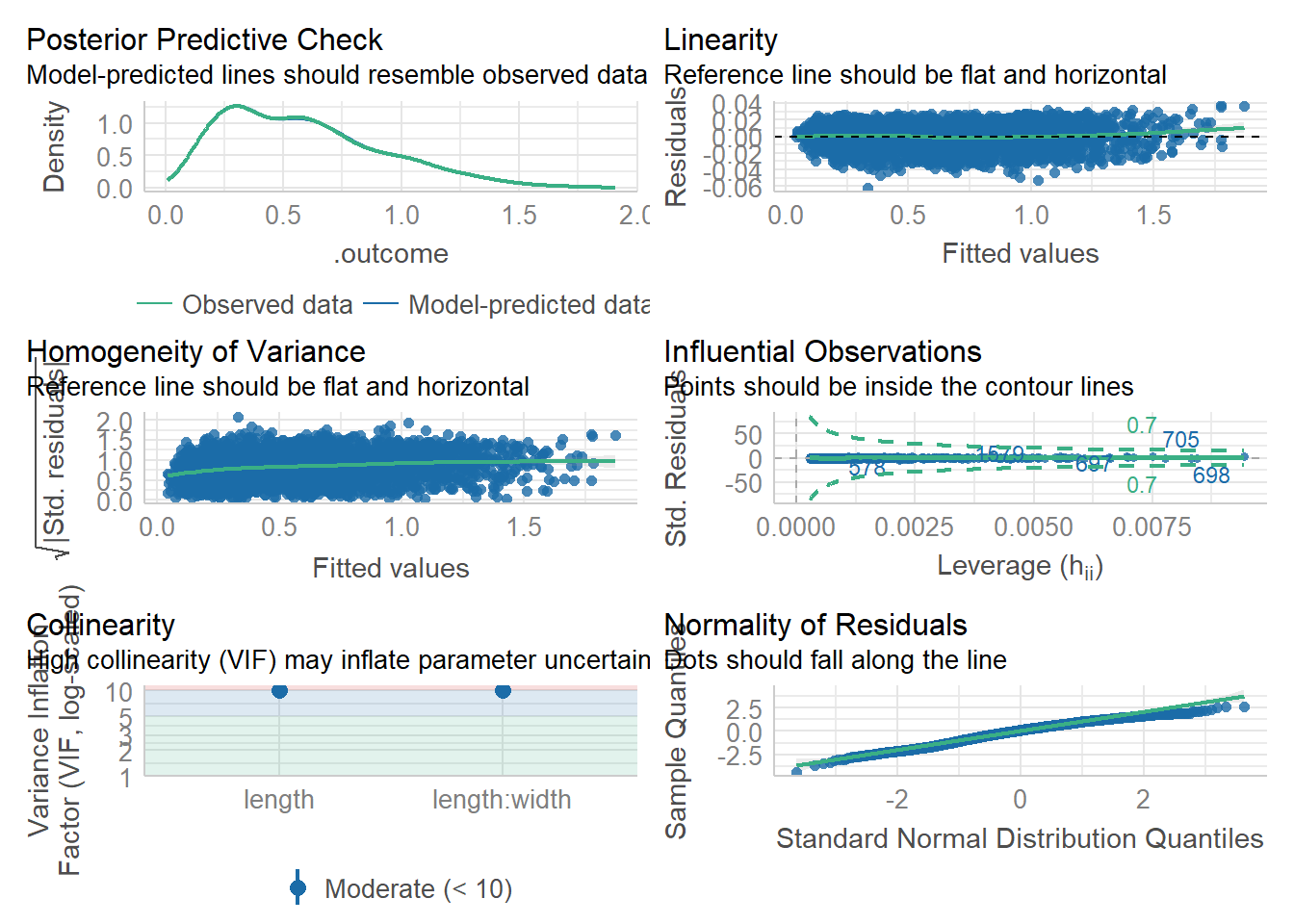

4 Predictions

library(ggpubr)

df_af <- 
  df_af |> 
  mutate(pred = predict(fit$finalModel))
get_ccc(df_af, area, pred)
##           r        pc    lwr_ci    upr_ci        bc
## 1 0.9991208 0.9991204 0.9990604 0.9991766 0.9999996


# 1:1 concordance plot
ggplot(df_af, aes(area, pred)) +
  geom_point(alpha = 0.2, color = "brown", size = 3) +
  geom_abline(intercept = 0, slope = 1, color = "red", linewidth = 1) +
  coord_equal() +
  xlim(c(0, 2)) +
  ylim(c(0, 2)) +
  labs(y = expression(Área~foliar~observada~(cm^2~folha^{-1})),
       x = expression(Área~foliar~predita~(cm^2~folha^{-1}))) +
  theme_bw(base_size = 16)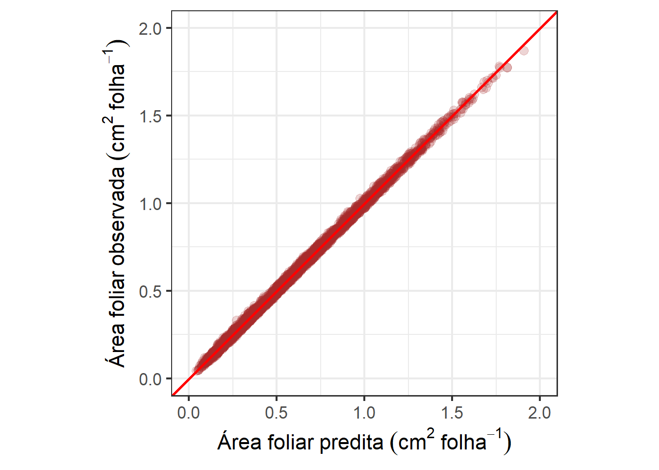

ggsave("figs/pred_af.jpg", dpi = 600)