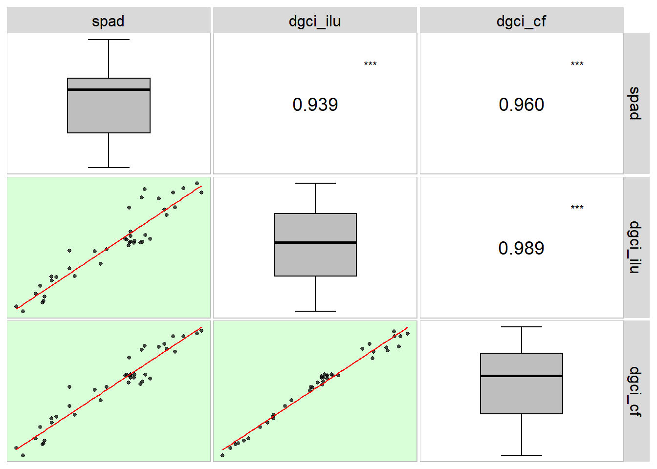
09: Relação entre SPAD e o índice DGCI em folhas de linho obtido em diferentes condições de iluminação

% Analysis

1 Libraries

To reproduce the examples of this material, the R packages the following packages are needed.

library(rio)
library(tidyverse)
library(metan)
library(pliman)
library(forcats)

2 Data

spad <- import("data/valor_spaad.xlsx")

3 DGCI

3.1 Imagem iluminada

img <- image_import("figs/dgci_ilum.jpg")

res_ilu <-
  analyze_objects_shp(img,
                      nrow = 4,
                      ncol = 10,
                      index = "B",
                      watershed = FALSE,
                      plot = FALSE,
                      pixel_level_index = TRUE,
                      object_index = "DGCI")
plot(img)
plot_measures(res_ilu, measure = "DGCI", digits = 3)
plot(res_ilu$shapefiles)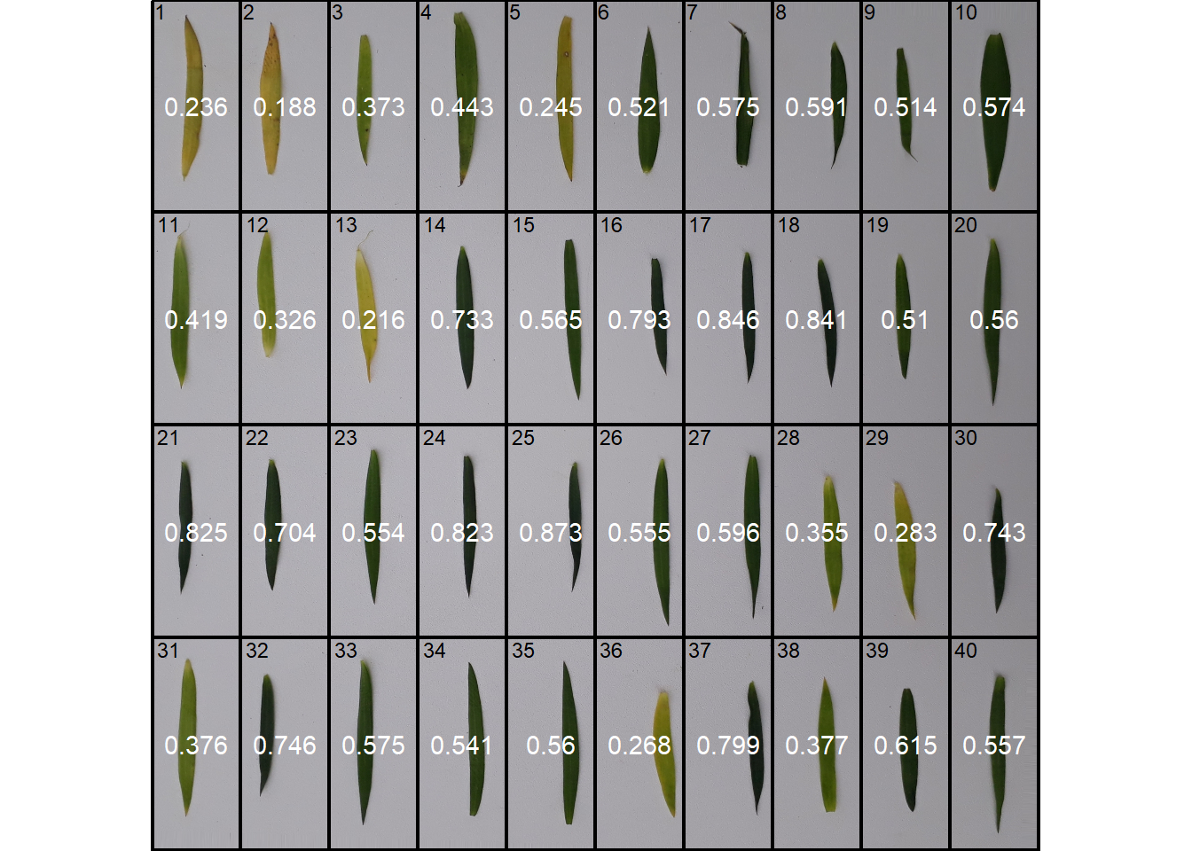

dgci_ilu <- res_ilu$object_index |> select(-id) |> rename(dgci_ilu = DGCI)

3.2 Interior, com flash

img <- image_import("figs/dgci_cf.jpg")

res_cf <-
  analyze_objects_shp(img,
                      nrow = 4,
                      ncol = 10,
                      index = "B",
                      watershed = FALSE,
                      plot = FALSE,
                      pixel_level_index = TRUE,
                      object_index = "DGCI")
plot(img)
plot_measures(res_cf, measure = "DGCI", digits = 3)
plot(res_cf$shapefiles)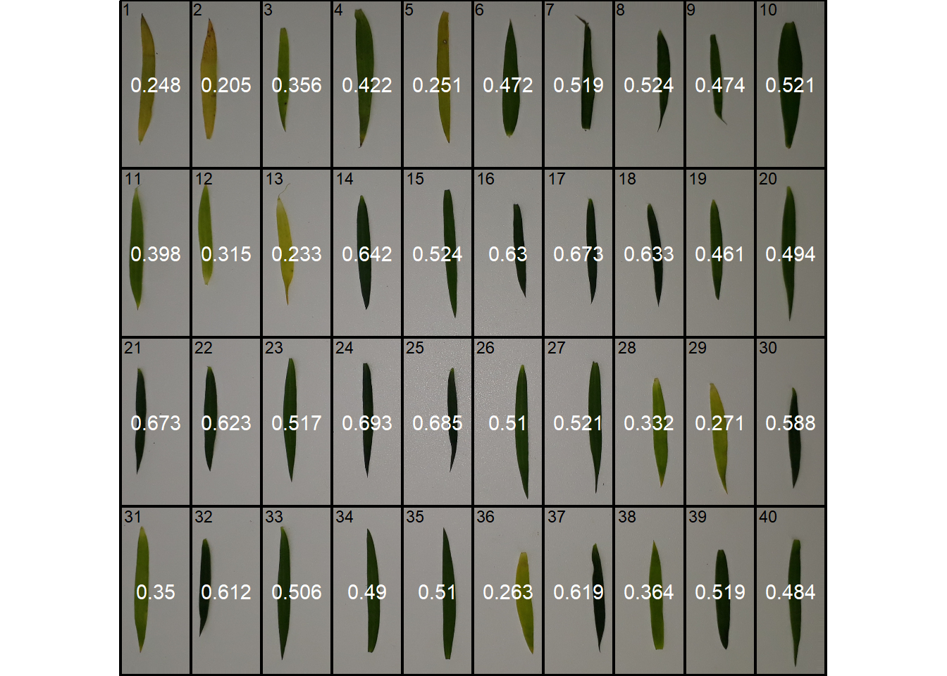

dgci_cf <- res_cf$object_index |> select(-id) |> rename(dgci_cf = DGCI)

4 Juntar os dados

df_spad <- 
  reduce(list(spad, dgci_ilu, dgci_cf), left_join) |> 
  mutate(condicao = ifelse(dgci_ilu < 0.5, "DGCI < 0,5", "DGCI >= 0,5"))

# export(df_spad, "data/df_spad.xlsx")

5 Correlação

corr_plot(df_spad, smooth = TRUE, confint = FALSE, digits = 3, diag.type = "boxplot")

ggsave("figs/dgci_cor.jpg",
       width = 5,
       height = 5)

6 Regressão

6.1 Gráfico

ggplot(df_spad, aes(dgci_cf, dgci_ilu, fill = condicao)) +
  geom_point(size = 5, color = "black", shape = 21, alpha = 0.8) +
  geom_smooth(method = "lm", se = FALSE, color = "red") +
  geom_abline(intercept = 0, slope = 1) +
  scale_x_continuous(limits = c(0, 1)) +
  scale_y_continuous(limits = c(0, 1)) +
  theme_bw(base_size = 19) +
  theme(panel.grid.minor = element_blank()) +
  labs(x = "DGCI com flash",
       y = "DGCI iluminado",
       color = "",
       fill = "") +
  theme(legend.position = "bottom") +
  scale_fill_manual(values = c("yellow", "darkgreen")) +
  coord_fixed()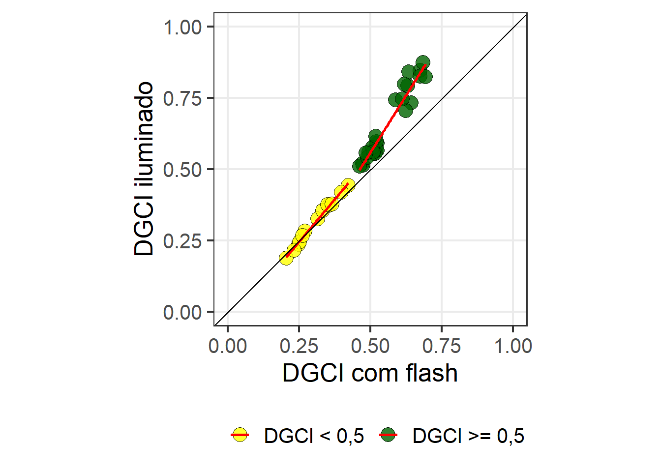

ggsave("figs/dgci_regressao.jpg",
       width = 6,
       height = 6)

6.2 Coeficientes

coefs_dgci <- 
  df_spad |> 
  group_by(condicao) %>% 
  doo(~lm(dgci_cf ~ dgci_ilu, data = .) |> broom::tidy())  

# export(coefs_dgci, "data/coefs_dgci.xlsx")

6.3 Densidade

dist_ilum <- 
  res_ilu[["object_rgb"]] |> 
  select(h, s, b, DGCI)

dist_cf <- 
  res_cf[["object_rgb"]] |> 
  select(h, s, b, DGCI)

df_hist <- 
  rbind_fill_id(dist_ilum, dist_cf, .id = "condicao") |> 
  mutate(amarelado = ifelse(DGCI < 0.5, "DGCI < 0,5", "DGCI >= 0,5"))

df_histp <- 
  df_hist |> 
  select(-DGCI) |> 
  pivot_longer(-c(condicao, amarelado)) |> 
  remove_rows_na() |> 
  mutate(name = fct_relevel(name, "h", "s", "b"))

ggplot(df_histp, aes(x = value, fill = amarelado)) +
  geom_density(alpha = 0.6) +
  facet_grid(condicao~name, scales = "free") +
  theme_bw(base_size = 20) +
  labs(x = "Valor observado",
       y = "Densidade",
       fill = "") +
  theme(legend.position = "bottom",
        panel.grid.minor = element_blank()) +
  scale_fill_manual(values = c("yellow", "darkgreen"))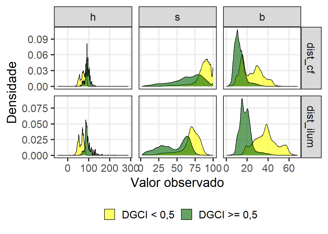

ggsave("figs/dgci_density.jpg",
       width = 10,
       height = 7)