08: Índices FAI-BLUP e MGIDI na seleção de genótipos de linho
% Analysis
1 Libraries
To reproduce the examples of this material, the R packages the following packages are needed.
2 Dados
3 Índice MGIDI
3.1 Sem pesos
mod_mgidi <-
  df |>
  mgidi(ideotype = c("l, h, h, h, h, h, h,  h, h"),
        SI = 25)
##
## -------------------------------------------------------------------------------
## Principal Component Analysis
## -------------------------------------------------------------------------------
## # A tibble: 9 × 4
##   PC    Eigenvalues `Variance (%)` `Cum. variance (%)`
##   <chr>       <dbl>          <dbl>               <dbl>
## 1 PC1          4.43          49.2                 49.2
## 2 PC2          1.72          19.1                 68.3
## 3 PC3          1.03          11.4                 79.8
## 4 PC4          0.94          10.4                 90.2
## 5 PC5          0.62           6.86                97.1
## 6 PC6          0.23           2.56                99.6
## 7 PC7          0.02           0.24                99.9
## 8 PC8          0.01           0.11               100.
## 9 PC9          0              0.02               100
## -------------------------------------------------------------------------------
## Factor Analysis - factorial loadings after rotation-
## -------------------------------------------------------------------------------
## # A tibble: 9 × 6
##   VAR     FA1   FA2   FA3 Communality Uniquenesses
##   <chr> <dbl> <dbl> <dbl>       <dbl>        <dbl>
## 1 cp     0.13 -0.13  0.78        0.65         0.35
## 2 nc    -0.9   0.13 -0.32        0.93         0.07
## 3 ng    -0.93 -0.12 -0.27        0.95         0.05
## 4 areac -0.55 -0.18  0.31        0.44         0.56
## 5 nr    -0.32 -0.18 -0.67        0.58         0.42
## 6 mc    -0.95  0.11 -0.25        0.97         0.03
## 7 rgpla -0.95  0.12 -0.23        0.97         0.03
## 8 ngcap -0.18 -0.92  0.08        0.88         0.12
## 9 mmg   -0.24  0.86  0.06        0.81         0.19
## -------------------------------------------------------------------------------
## Comunalit Mean: 0.7976177
## -------------------------------------------------------------------------------
## Selection differential
## -------------------------------------------------------------------------------
## # A tibble: 9 × 8
##   VAR   Factor      Xo      Xs       SD SDperc sense     goal
##   <chr> <chr>    <dbl>   <dbl>    <dbl>  <dbl> <chr>    <dbl>
## 1 nc    FA1     33.5    57.6    24.0     71.8  increase   100
## 2 ng    FA1    216.    394.    178.      82.3  increase   100
## 3 areac FA1      0.394   0.423   0.0290   7.35 increase   100
## 4 mc    FA1      1.64    3.07    1.43    87.7  increase   100
## 5 rgpla FA1      1.22    2.34    1.12    92.3  increase   100
## 6 ngcap FA2      6.47    6.90    0.431    6.67 increase   100
## 7 mmg   FA2      5.60    6.11    0.511    9.14 increase   100
## 8 cp    FA3     27.6    26.8    -0.775   -2.81 decrease   100
## 9 nr    FA3      1.29    1.62    0.337   26.2  increase   100
## ------------------------------------------------------------------------------
## Selected genotypes
## -------------------------------------------------------------------------------
## G48 G228 G4 G13 G222 G9 G31 G10 G23 G14 G36 G17 G21 G3 G29 G215
## -------------------------------------------------------------------------------
3.2 Com pesos
mod_mgidi_peso <-
  df |>
  mgidi(ideotype = c("l, h, h, h, h, h, h,  h, h"),
        weights = c(2, 5, 5, 1, 1, 5, 5, 2, 2),
        SI = 25)
##
## -------------------------------------------------------------------------------
## Principal Component Analysis
## -------------------------------------------------------------------------------
## # A tibble: 9 × 4
##   PC    Eigenvalues `Variance (%)` `Cum. variance (%)`
##   <chr>       <dbl>          <dbl>               <dbl>
## 1 PC1          4.43          49.2                 49.2
## 2 PC2          1.72          19.1                 68.3
## 3 PC3          1.03          11.4                 79.8
## 4 PC4          0.94          10.4                 90.2
## 5 PC5          0.62           6.86                97.1
## 6 PC6          0.23           2.56                99.6
## 7 PC7          0.02           0.24                99.9
## 8 PC8          0.01           0.11               100.
## 9 PC9          0              0.02               100
## -------------------------------------------------------------------------------
## Factor Analysis - factorial loadings after rotation-
## -------------------------------------------------------------------------------
## # A tibble: 9 × 6
##   VAR     FA1   FA2   FA3 Communality Uniquenesses
##   <chr> <dbl> <dbl> <dbl>       <dbl>        <dbl>
## 1 cp     0.13 -0.13  0.78        0.65         0.35
## 2 nc    -0.9   0.13 -0.32        0.93         0.07
## 3 ng    -0.93 -0.12 -0.27        0.95         0.05
## 4 areac -0.55 -0.18  0.31        0.44         0.56
## 5 nr    -0.32 -0.18 -0.67        0.58         0.42
## 6 mc    -0.95  0.11 -0.25        0.97         0.03
## 7 rgpla -0.95  0.12 -0.23        0.97         0.03
## 8 ngcap -0.18 -0.92  0.08        0.88         0.12
## 9 mmg   -0.24  0.86  0.06        0.81         0.19
## -------------------------------------------------------------------------------
## Comunalit Mean: 0.7976177
## -------------------------------------------------------------------------------
## Selection differential
## -------------------------------------------------------------------------------
## # A tibble: 9 × 8
##   VAR   Factor      Xo      Xs       SD SDperc sense     goal
##   <chr> <chr>    <dbl>   <dbl>    <dbl>  <dbl> <chr>    <dbl>
## 1 nc    FA1     33.5    59.8    26.2    78.3   increase   100
## 2 ng    FA1    216.    390.    174.     80.3   increase   100
## 3 areac FA1      0.394   0.423   0.0286  7.24  increase   100
## 4 mc    FA1      1.64    3.12    1.48   90.8   increase   100
## 5 rgpla FA1      1.22    2.36    1.15   94.1   increase   100
## 6 ngcap FA2      6.47    6.51    0.0449  0.694 increase   100
## 7 mmg   FA2      5.60    6.50    0.906  16.2   increase   100
## 8 cp    FA3     27.6    26.5    -1.09   -3.95  decrease   100
## 9 nr    FA3      1.29    1.69    0.400  31.0   increase   100
## ------------------------------------------------------------------------------
## Selected genotypes
## -------------------------------------------------------------------------------
## G228 G4 G48 G13 G222 G31 G9 G36 G28 G29 G10 G21 G23 G41 G14 G17
## -------------------------------------------------------------------------------
4 FAI-BLUP
mod_fai <-
  df |>
  column_to_rownames("gen") |>
  fai_blup(DI = c("min, max, max, max, max, max, max, max, max"),
           UI = c("max, min, min, min, min, min, min, min, min"),
           SI = 25)
##
## -----------------------------------------------------------------------------------
## Principal Component Analysis
## -----------------------------------------------------------------------------------
##     eigen.values cumulative.var
## PC1         4.43          49.23
## PC2         1.72          68.31
## PC3         1.03          79.76
## PC4         0.94          90.20
## PC5         0.62          97.06
## PC6         0.23          99.63
## PC7         0.02          99.87
## PC8         0.01          99.98
## PC9         0.00         100.00
##
## -----------------------------------------------------------------------------------
## Factor Analysis
## -----------------------------------------------------------------------------------
##         FA1   FA2   FA3 comunalits
## cp    -0.13  0.13  0.78       0.65
## nc    -0.90  0.13  0.32       0.93
## ng    -0.93 -0.12  0.27       0.95
## areac -0.55 -0.18 -0.31       0.44
## nr    -0.32 -0.18  0.67       0.58
## mc    -0.95  0.11  0.25       0.97
## rgpla -0.95  0.12  0.23       0.97
## ngcap -0.18 -0.92 -0.08       0.88
## mmg   -0.24  0.86 -0.06       0.81
##
## -----------------------------------------------------------------------------------
## Comunalit Mean: 0.7976177
## Selection differential
## -----------------------------------------------------------------------------------
##     VAR Factor          Xo          Xs          SD     SDperc    sense goal
## 1    nc      1  33.5151515  42.3125000  8.79734848  26.248870 increase  100
## 2    ng      1 216.0757576 286.3750000 70.29924242  32.534535 increase  100
## 3 areac      1   0.3942657   0.4272672  0.03300152   8.370376 increase  100
## 4    mc      1   1.6351515   2.2025000  0.56734848  34.696998 increase  100
## 5 rgpla      1   1.2174242   1.6550000  0.43757576  35.942750 increase  100
## 6 ngcap      2   6.4669836   6.8869142  0.41993055   6.493453 increase  100
## 7   mmg      2   5.5972761   6.0208227  0.42354665   7.567014 increase  100
## 8    cp      3  27.5560606  22.8562500 -4.69981061 -17.055452 decrease  100
## 9    nr      3   1.2878788   1.0000000 -0.28787879 -22.352941 increase    0
##
## -----------------------------------------------------------------------------------
## Selected genotypes
## G48 G31 G9 G28 G8 G35 G5 G17 G15 G21 G12 G222 G30 G228 G23 G13
## -----------------------------------------------------------------------------------
5 Ganhos
5.1 Individuais
gmgidisp <-
  gmd(mod_mgidi) |>
  select(VAR, sense, mgidi_sp = SDperc)

gmgidicp <-
  gmd(mod_mgidi_peso) |>
  select(VAR,  mgidi_cp = SDperc)

gfai <-
  gmd(mod_fai) |>
  select(VAR, fai = SDperc)

bind <-
  reduce(list(gmgidisp, gmgidicp, gfai), left_join) |>
  pivot_longer(-c(VAR, sense)) |>
  mutate(sense = ifelse(sense == "decrease", "Reduzir", "Aumentar"))


facet_labels <- c("FAI-BLUP", "MGIDI com peso", "MGIDI sem peso")
names(facet_labels) <- c("fai", "mgidi_cp", "mgidi_sp")

ggplot(bind, aes(value, VAR)) +
  geom_col(position = position_dodge(),
           aes(fill = sense),
           width = 1,
           linewidth = 0.1,
           color = "black") +
  geom_text(aes(label = round(value, 2),
                hjust = ifelse(value > 0, -0.1, 1.1)),
            size = 4) +
  facet_wrap(~name,
              labeller = labeller(name = facet_labels)) +
  theme_bw(base_size = 18) +
  theme(axis.text = element_text(size = 12, color = "black"),
        axis.ticks.length = unit(0.2, "cm"),
        panel.grid.minor = element_blank(),
        legend.title = element_blank(),
        # legend.position = "bottom",
        panel.spacing.x = unit(0, "cm")) +
  scale_fill_hue(direction = -1) +
  geom_vline(xintercept = 0, linetype = 1, linewidth = 1) +
  scale_x_continuous(expand = expansion(c(0.4, 0.4))) +
  labs(y = "Caracteres avaliados",
       x = "Diferencial de seleção (%)") +
  geom_vline(xintercept = 0)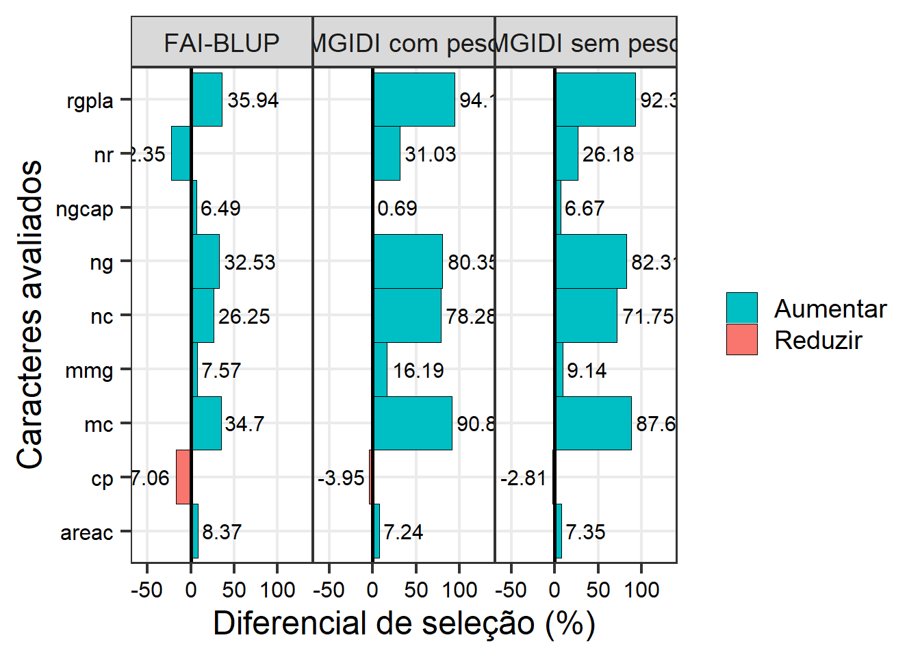
ggsave("figs/gains_mgidi_fai.jpg",
       width = 10,
       height = 5)
5.2 Totais
tot_fai <- mod_fai[["total_gain"]][["ID1"]] |> mutate(indice = "FAI-BLUP")
tot_mgidi_cp <- mod_mgidi_peso$stat_gain |> mutate(indice = "MGIDI com peso")
tot_mgidi_sp <- mod_mgidi$stat_gain |> mutate(indice = "MGIDI sem peso")

totais <-
  bind_rows(tot_fai, tot_mgidi_cp, tot_mgidi_sp) |>
  select(sense, max, sum, indice) |>
  pivot_longer(cols = max:sum) |>
    mutate(sense = ifelse(sense == "decrease", "Reduzir", "Aumentar"))

facet_labels <- c("Diferenciais máximos", "Soma dos diferenciais")
names(facet_labels) <- c("max", "sum")

ggplot(totais, aes(indice, value)) +
  geom_col(aes(fill = sense),
           position = position_dodge(width = 1)) +
  facet_wrap(~name,
             # scales = "free",
             labeller = labeller(name = facet_labels)) +
  theme_bw(base_size = 18) +
  theme(axis.text = element_text(size = 12, color = "black"),
        axis.text.x = element_text(angle = 30, vjust = 1, hjust = 1),
        axis.ticks.length = unit(0.2, "cm"),
        panel.grid.minor = element_blank(),
        legend.title = element_blank(),
        # legend.position = "bottom",
        panel.spacing.x = unit(0, "cm")) +
    scale_fill_hue(direction = -1) +
  labs(x = "Índices",
       y = "Diferencial de seleção (%)") +
  geom_text(aes(label = round(value, 2),
                vjust = ifelse(value < 0, 1.2, -1),
                hjust = ifelse(value > 0, 1, 0))) +
  scale_y_continuous(expand = expansion(0.1)) +
  geom_hline(yintercept = 0,
             linewidth = 0.9)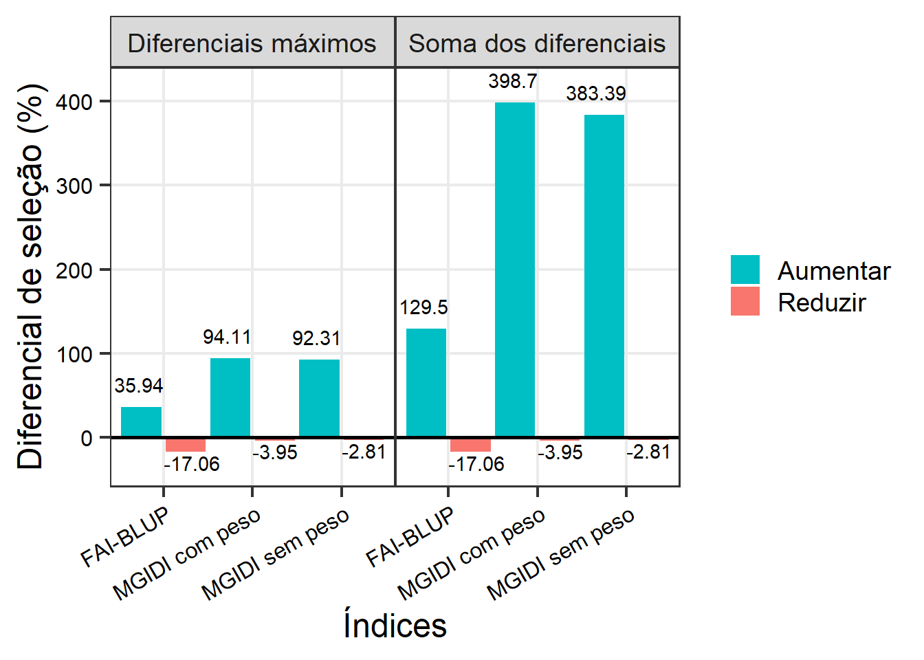
ggsave("figs/total_gains_mgidi_fai.jpg",
       width = 9,
       height = 7)
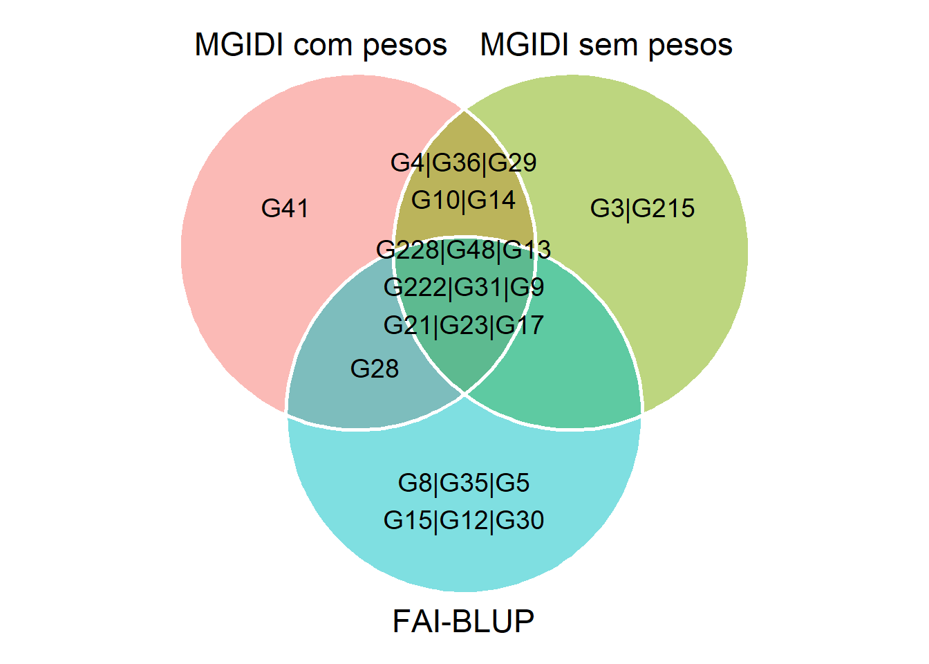
6 Venn plot
7 Section info
sessionInfo()
## R version 4.2.2 (2022-10-31 ucrt)
## Platform: x86_64-w64-mingw32/x64 (64-bit)
## Running under: Windows 10 x64 (build 22621)
##
## Matrix products: default
##
## locale:
## [1] LC_COLLATE=Portuguese_Brazil.utf8  LC_CTYPE=Portuguese_Brazil.utf8
## [3] LC_MONETARY=Portuguese_Brazil.utf8 LC_NUMERIC=C
## [5] LC_TIME=Portuguese_Brazil.utf8
##
## attached base packages:
## [1] stats     graphics  grDevices utils     datasets  methods   base
##
## other attached packages:
##  [1] metan_1.18.0    lubridate_1.9.2 forcats_1.0.0   stringr_1.5.0
##  [5] dplyr_1.1.2     purrr_1.0.1     readr_2.1.4     tidyr_1.3.0
##  [9] tibble_3.2.1    ggplot2_3.4.2   tidyverse_2.0.0 rio_0.5.29
##
## loaded via a namespace (and not attached):
##  [1] jsonlite_1.8.7      splines_4.2.2       cellranger_1.1.0
##  [4] yaml_2.3.7          ggrepel_0.9.3       numDeriv_2016.8-1.1
##  [7] pillar_1.9.0        lattice_0.20-45     glue_1.6.2
## [10] digest_0.6.33       RColorBrewer_1.1-3  polyclip_1.10-4
## [13] minqa_1.2.5         colorspace_2.1-0    htmltools_0.5.5
## [16] Matrix_1.6-0        plyr_1.8.8          pkgconfig_2.0.3
## [19] haven_2.5.3         patchwork_1.1.2     scales_1.2.1
## [22] tweenr_2.0.2        openxlsx_4.2.5.2    tzdb_0.4.0
## [25] lme4_1.1-34         ggforce_0.4.1       timechange_0.2.0
## [28] generics_0.1.3      farver_2.1.1        withr_2.5.0
## [31] cli_3.6.1           magrittr_2.0.3      readxl_1.4.3
## [34] evaluate_0.21       GGally_2.1.2        fansi_1.0.4
## [37] nlme_3.1-160        MASS_7.3-60         foreign_0.8-83
## [40] textshaping_0.3.6   tools_4.2.2         data.table_1.14.8
## [43] hms_1.1.3           lifecycle_1.0.3     munsell_0.5.0
## [46] zip_2.3.0           compiler_4.2.2      systemfonts_1.0.4
## [49] rlang_1.1.1         grid_4.2.2          nloptr_2.0.3
## [52] rstudioapi_0.15.0   htmlwidgets_1.6.2   labeling_0.4.2
## [55] rmarkdown_2.23      boot_1.3-28         gtable_0.3.3
## [58] lmerTest_3.1-3      reshape_0.8.9       curl_5.0.1
## [61] R6_2.5.1            knitr_1.43          fastmap_1.1.1
## [64] utf8_1.2.3          mathjaxr_1.6-0      ragg_1.2.5
## [67] stringi_1.7.12      Rcpp_1.0.11         vctrs_0.6.3
## [70] tidyselect_1.2.0    xfun_0.39